
Abstract
This study analyzes signalized-intersection performance in Bumi Serpong Damai using calibrated VISSIM microsimulation based on peak-hour traffic, geometric data, and signal-timing parameters. Model accuracy was ensured through iterative behavioural calibration and R² validation. Optimisation scenarios involving revised phase plans and green-time allocation produced clear improvements, including reduced delay, stop frequency, queue length, and emissions. The results demonstrate the effectiveness of data-driven signal-timing strategies and provide a transferable framework for intersection optimisation in rapidly growing urban areas.
Keywords: intersection, microsimulation, optimization, reduce, vissim
Outline
1. Introduction
Population growth aligns with increased economic activity and mobility1,2). Existing transportation facilities must be evaluated to ensure their capacity to accommodate the community's growing mobility needs each year. The road network is part of the transportation system and represents essential infrastructure. Hence, road network disruptions can bring social, economic, political, and environmental impacts3,4). Traffic system modeling is critical in transportation engineering5).
Traffic congestion is a prevalent issue in numerous urban areas around Indonesia6). The increase in private vehicle ownership7) and population growth8) These are the main causes of rising traffic volumes, which can increase fuel consumption and decrease vehicle speed9,10). Meanwhile, intersections, as part of the road network, become conflict points where multiple vehicle flow directions converge. This reduces the intersection’s capacity and often leads to accidents11). Signalised intersections can reduce traffic conflicts12), increasing road capacity while decreasing vehicle operating costs and travel time.
Additionally, traffic from minor roads may face challenges in merging, especially if the flow from major roads is relatively high, causing significant delays for vehicles from minor roads13). Previous studies indicate that the risk of accidents for road users and pedestrians at unsignalized intersections is relatively high due to the absence of traffic signal regulation, leading to increasingly uncontrolled and complicated traffic flow14).
Modern cities have essential infrastructure systems that enhance activities to support the well-being of residents15,16). The increasing population and number of vehicles lead to higher vehicle movement and intensified activity at intersections17–20), contributing to increased emissions21,22). High economic growth has resulted in higher travel demand22). The rate of urbanization is one of the causes of traffic congestion23–25). The increase in the number of vehicles poses a problem faced by cities worldwide26,27). The transportation sector is one of the main sources of air pollution, contributing 25–30 percent of global CO2 emissions28,29), with most transport-related emissions originating from road transport30). Pollution from vehicle emissions has adverse effects on health31), being the primary cause of 3.3 million deaths annually worldwide32) and ranking among the top causes of death globally, with 50,000 deaths annually in the UK alone33). Traffic congestion increases the risk of accidents34,35). It also leads to wasted fuel consumption, higher vehicle operating costs, extended travel times, deteriorated air quality, and compromised traffic safety. Prolonged vehicle delays at intersections cause these problems, so improvements to transportation infrastructure's efficiency and functionality are necessary36).
Intersections are a vital part of the transportation system, with their disruptions potentially causing social, health, economic, and environmental hazards. Intersections can be likened to the arteries of a vast and complex organism, transferring resources from one place to another. As part of intersection control, traffic lights are essential for regulating urban transportation networks37). Intersections require a well-designed traffic-light system. In some cases, where traffic volume is low, adjusting traffic signals may not need elaborate strategies; however, during peak hours when traffic density increases, particularly on one side of the intersection, effective traffic light control becomes crucial. Traffic lights are essential for managing traffic flow, improving service levels, and ensuring road user safety. While analytical methods offer initial performance insights, their simplifying assumptions often fail to capture the complexity of heterogeneous traffic compositions, variable driver responses, and dynamic interactions at the movement level38). As a result, microsimulation models have become the dominant tool for evaluating intersection performance, enabling detailed representation of behaviour-based parameters, saturation flow variability, and phase-level control logic39).
Despite the widespread adoption of microsimulation, several key methodological gaps remain. First, many studies continue to rely on default or partially calibrated behavioural parameters, which can compromise simulation fidelity, particularly in mixed-traffic or context-sensitive conditions40). Second, optimisation efforts often focus on generic timing strategies without fully incorporating geometric constraints, turning-movement asymmetries, or land-use-driven demand patterns that influence signal performance in fast-developing suburban corridors41). Third, although emission modeling is increasingly embedded in simulation platforms, the linkage between operational improvements and environmental outcomes especially in stop and go dominated corridors remains underexamined42). Vissim is a transportation software for simulating microscopic multimodal traffic, including public transportation and pedestrians. The input models include cars, freight transport, buses, heavy rail, trams, LRT, motorcycles, bicycles, and pedestrians. These modes can interact with one another. Users of this software can model various geometric configurations and road user behaviors in transportation systems. The analysis results from the Vissim model can predict increases in vehicle flow and speed, enabling the evaluation of performance improvement signalised intersections in terms of delays and travel times. A proper understanding of vehicle movements within the road network, including effective traffic management at intersections, will aid in formulating urban transport policies. Vissim and other software, such as Transyt, SimTraffic, Vissum, S-Paramics, and SISTM, are commonly used for microanalysis in transportation simulations. One of the advantages of Vissim microsimulation software is its flexibility in modelling mixed traffic flows, which closely resemble traffic conditions in Indonesia4). The Foresta BSD signalised intersection is located in South Tangerang City, within a central business district featuring offices, shopping centres, and residential areas, which generate high traffic volumes. Long vehicle queues are typically observed at the Foresta BSD intersection during morning and evening peak hours. This increases transportation costs for road users and reduces the region's economic competitiveness if not properly addressed. This highlights that the current road infrastructure is insufficient to handle the vehicle load43). Therefore, finding effective solutions to manage congestion appropriately while benefiting the community is crucial. This study aims to evaluate the operational performance of the Foresta BSD signalised intersection under existing conditions by assessing indicators such as delay, queue length, number of stops, and level of service. Using PTV VISSIM microsimulation, the study further seeks to develop and test several signal-timing and phase-optimisation scenarios, and to compare their impacts on traffic performance and vehicle emissions. The ultimate objective is to identify an optimisation strategy that can improve intersection service, enhance travel efficiency, and support better environmental quality in the future.
2. Literature Review
2.1. Intersection
Intersections are locations where traffic from different directions meets, creating potential conflicts between opposing flows and, consequently, congestion12). Based on their control type, intersections can be classified into signalised and unsignalized. At unsignalized intersections, there are no traffic lights, and right-of-way is typically governed by signs or priority rules, so drivers must slow down or stop briefly before crossing. At signalised intersections, traffic lights and other control devices regulate the movement of vehicles, pedestrians, and cyclists. Figure 1 illustrates a typical four-leg signalised intersection used in this study. The four approaches are numbered 1–4, and each approach is controlled by a three-
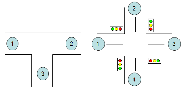
aspect (red–amber–green) traffic signal head installed upstream of the stop line. An increase in traffic density at such intersections leads to longer delay times and reduced safety, comfort, and overall level of service. Delay time refers to the average time vehicles must wait to pass through the intersection; the higher the delay time, the longer the overall travel time.
2.2. Traffic Modelling
SimTraffic Synchro 7 is another software used in transportation, especially in traffic engineering. This software may not be well known, particularly in Indonesia, especially for those who rarely use it in transportation. This software allows us to model road forms, from simpler straight roads to signalized or non-signalized intersections, roundabouts, flyovers, and even the coordination of all highways in a city. Users can simply sketch the road and enter the volume, movement, number of lanes, and other basic data. Then, users can calculate the degree of saturation and the emission gases produced by vehicle data.
CORSIM is a micro-scopic traffic simulation software capable of modelling surface roads, expressways, highways, and integrated works, including segments, weavers, combined/diverging lanes, and intersections with stop signs and traffic signals. It simulates traffic and traffic control systems using vehicle and driver behaviour models. CORSIM provides both animated and static graphics of network traffic44).
2.3. PTV Vissim
System modelling is an approach to describe the relationship between transportation infrastructure and traffic flow in the current condition45). PTV VISSIM is a microscopic simulation program based on time and behaviour, developed for urban traffic models46,47). These programs analyse traffic operations under the constraints of road linear configuration, traffic composition, stopping places, and others41). This software helps evaluate various transportation engineering alternatives and the most effective design level. There are 168 parameters embedded in VISSIM. Based on these parameters, several were selected under heterogeneous traffic conditions in Indonesia to develop a model according to the field circumstances. The parameters chosen for modelling are4):
a)Minimum headway is the minimum distance available for the vehicle in front to change lanes or overtake. The default value ranges from 0.5 to 3 seconds.
b)Lane Change Rule is the driver’s behavior model when passing through heterogeneous traffic, which is very suitable for free lane-change models that allow the vehicle to prepare freely.
c)Lateral Minimum Distance is the driver’s safe distance alongside another vehicle. This parameter is divided into two parts: the distance travelled at 0 km/h and at 50 km/h. The value of this parameter varies with speed, with the default value ranging from 0.2 to 1 m.
d)Standstill Distance in Front of Obstacle is a parameter for the safe distance when the vehicle will stop due to a stopped vehicle or deceleration due to obstacles in meters (m).
e)Observed Vehicles in Front indicates the number of vehicles the driver pays attention to when intending to move or react. The default values for this parameter are one, two, three, and four vehicle units.
f)Additive Factor Security is an additional value as a parameter for the safe distance the vehicle will stop. The recommended default value for this parameter is 0.45 - 2.
g)Multiplicative Factor Security is a factor that multiplies the safe distance of the vehicle when it is about to stop. The default values range from 1 to 3.
h)Overtaking Same Lane is the behaviour of vehicle drivers who want to overtake in the same lane from either the right or left sides.
i)Desired Lateral Position is the vehicle's position in the lane, meaning the vehicle can be on the left or right side of other cars.
j)Safety Distance Reduction is the safe distance between the vehicle in front and behind, or the gap and clearing distance between cars. This is a decisive parameter because each traffic condition has a different safe distance, with the study's default value being 0.6m.
Based on these parameter configurations, calibration and validation works, microsimulation applications, including PTV VISSIM software, have been recently used to evaluate signalised intersection performances, especially in Indonesian cities or other developing countries42). Traditionally, intersection performance measurements are based on PKJI/MKJI- Look–and- say/GPL-based measures such as saturation flow, delay, queue lengths and level-of-service parameters. Nevertheless, PTV VISSIM micro-simulation allows a more meaningful insight into the operational performance of intersections, particularly in heterogeneous traffic conditions43).
Internationally, there are numerous studies use PTV VISSIM to explore and optimise signalised control on congested intersections, including developed cities as well as developing countries with mixed traffic. Studies have indicated that changes in the cycle times, split allocation time among phases and more flexible phase settings can reduce the average delay levels, decrease the number of stops in vehicular flow as well as improve traffic flow during peak hours44). This approach is often combined with corridor and network performance evaluations to analyse how changes in signal settings at one location (i.e., intersection) can affect the performance of downstream segments and intersections.
In Indonesia, the use of PTV VISSIM in traffic engineering studies is growing, especially in the case of urban road network signalised intersections that are subjected to fast increases in road traffic level. Case studies in large cities and their surrounding areas show that combining traditional PKJI/MKJI methods with microsimulation provides a more realistic representation of driver conduct and traffic interactions43). This phenomenon includes the effects of motorcycles, rapid onset disordered flow and non-uniform clustering45). The results also highlight that microsimulation is a necessary tool for analysis across various engineering scenarios, such as changes in signal phase settings, cycle time changes of the signals, if new approach lanes were added and if they were adequately marked or signaged.
Aside from operational performance metrics, such as delay and queue lengths, a few studies are starting to correlate intersection performance with vehicle emissions and consequently, air quality. Through the comparison of microsimulation results (e.g., speed, travel time, and stop-go patterns) with emission models, these studies suggest that the lack of coordination of signals operations may increase fuel consumption and pollutants emissions near intersections (The impact). For example, prolonging the red time or unbalancing green time distribution ratios among arms could lead to, a queue and higher acceleration-deceleration frequencies with degraded air quality for the region46). These findings underscore the importance of considering traffic performance metrics such as queues, in conjunction with energy and environmental impacts during signal setting design and evaluation.
Although a lot of work has been done on performance analysis at signalised intersections using microsimulation, few studies have dealt with the intersections in the newly developed areas, such as the Bumi Serpong Damai (BSD) area within South Tangerang City, experiencing substantial residential and commercial developments. In fact, there are few studies, that simultaneously assess the traffic performance and its implications in terms of vehicular emissions in relation to the surrounding feeder road network where this new development area is connected44,47,48). Therefore, in this study, we wish to contribute to the relevant work by investigating signalised intersections in Foresta BSD with PTV VISSIM and developing signal phase optimisation scenarios that can be evaluated for their effect on delays, stops and emissions. It contributes significantly to the traffic control and environmental conditions on this plateau.
3. Methodology
3.1. Research Location and Description
The Foresta BSD intersection (Figure 2) is one of the points that contribute to congestion in South Tangerang
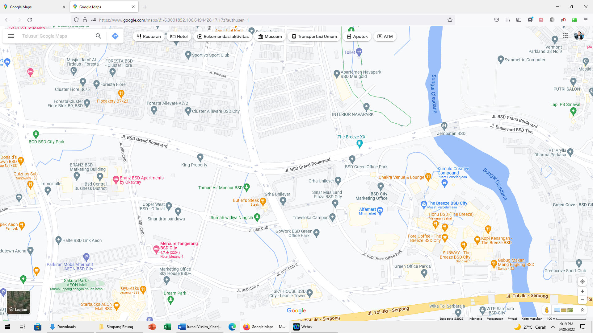
City. This intersection is close to the exit and entry access of the BSD toll road, so during peak hours, the condition of this intersection is very congested, compounded by its location, which is near shopping centres, offices, hospitals, and the central business district.
3.2. Research Stage
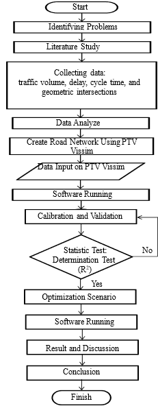
The first stage of this research is identifying problems at the research location. After that, a preliminary survey is conducted to assess the current conditions at the research location, including traffic conditions, observation points, and geometric characteristics of intersections, and to identify suitable observation points to support data collection48). Next, primary data are collected by surveying traffic volume, delay, cycle time, and geometric characteristics of intersections. Secondary data used includes population data and road classification data. Then, the data is analysed using VISSIM software to model the current intersection traffic and create a new simulation model that results in improved performance of the Forerstra BSD intersection, namely reducing delay times and the number of stops. The research stage flow chart is shown in Figure 3.
3.3. Data Collection
To build a simulation model using PTV VISSIM, several types of field data are required, including geometric road data, traffic volume, traffic composition, queue lengths, delays, and vehicle speeds. These data were collected at the Foresta BSD intersection and then used as inputs for the microsimulation model.
a)Road geometric data: This includes the width of the approach lanes, measured using a length gauge, and the number of lanes in each approach, which are recorded to determine the type of intersection.
b)Traffic volume: Traffic volume data were obtained through a manual traffic counting survey at the Foresta BSD intersection. Traffic variations are generally represented at hourly, daily, or seasonal scales; therefore, the timing of the survey depends on the study objective. To describe traffic
conditions during peak hours, the survey was conducted on a typical weekday (Thursday) from 06:00 to 18:00 WIB with 5–15 minutes intervals42). From these data, the morning and evening peak hours were identified and used to define the simulation period. Traffic volume and vehicle speed are essential inputs for evaluating road and intersection performance.
c)Composition of traffic: Through a traffic volume survey, vehicle types can be classified into light vehicles, motorcycles, heavy vehicles/buses, and non-motorized vehicles. This classification was later converted into traffic composition percentages and entered into VISSIM to represent heterogeneous (mixed) traffic conditions typical of Indonesian urban roads.
d)Queue length: This is defined as the length of the queue of vehicles in an approach and is expressed in meters. This is the distance from the car’s farthest point to the stop line. The number of vehicles that stop in each major or minor lane is calculated over specified time intervals, both in the morning and evening. To estimate the number of vehicle queues, the queue length measured on the approach is divided by 6 meters to get the number of cars in the queue48). This value is obtained by summing the safe distances between the vehicle ahead and behind, where the average vehicle length in Indonesia is about 4.7 meters.
e)Delay: Delay is the total average drag time experienced by a vehicle when passing through an intersection. The value of the delay affects the vehicle's travel time. The higher the delay, the longer the travel time. Delay is a measure of intersection performance representing each vehicle's average delay. Data collection is done by following a car through the intersection at an average speed, matching the speed of other vehicles in the flow during peak hours. The in-vehicle survey records the car's total time from the control point to the stop line. This survey was conducted several times during the observation to determine the average vehicle delay.
f)Vehicle speed: Vehicle speed is the average speed of a vehicle when passing through the intersection. This study used two approaches to determine the vehicle's speed. The first is recording the speed of several randomly selected cars approaching an intersection using a speed gun, and the second is recording the vehicle's speed by the surveyor, driving the car at a speed matching the average speed of other vehicles in the flow.
g)Survey Period: Data collection was carried out during peak hours because the aim of this research is to provide recommendations for handling signalized intersections in the Primavera Foresta BSD area during overcrowded conditions, which occur during peak hours.
3.4. Data Processing and Simulation Modelling Vissim
The intersection, the research object, is captured using aerial images via the Google Earth site to be modelled in VISSIM. The image is imported according to the expected scale to represent the actual road conditions, as shown below. Next, arrange the order of movement according to the order of priority, conflict markers, and vehicle stop lines.
a)Background import and scaling
A background image of the study location was imported into VISSIM. The image was scaled to match real-world distances to ensure that the geometric shapes and surrounding environmental conditions were consistent with the field.
b)Road network development
The road network was created by defining links and connectors that followed the background image. This process included modelling the approaches, exit legs, and internal connectors at the intersection to ensure that the network closely resembled the actual geometric conditions.
c)Route definition
Vehicle routes were created using Vehicle Routers to represent the actual movement patterns and turning proportions at the intersection. These routes follow the observed traffic flow directions (through, left-turn, right-turn) on each approach.
d)Vehicle type specification
Vehicle types in the model were defined according to the field survey, including heavy vehicles, light vehicles, motorcycles, and non-motorised vehicles. Each vehicle type was assigned appropriate physical and behavioural characteristics to reflect mixed traffic conditions.
e)Traffic volume input
Observed traffic volumes from the survey were input into the model using the Vehicle Input command for each approach. The input values correspond to peak-hour volumes for each movement and vehicle class.
f)Desired speed distribution
Vehicle speeds in the simulation were controlled using the Desired Speed Distribution command. The speed distributions were adjusted to align the simulated speeds with the measured field speeds, ensuring that the model realistically represented driver behaviour.
g)Signal control configuration
The traffic signal phases were configured in the model using the Signal Controller command to match the existing field settings at the Foresta BSD intersection. This included defining cycle length, green, amber, and red times, as well as phase sequences for each approach.
h)Driving behaviour settings
Driver behaviour parameters were adjusted to represent typical driving patterns in Indonesia. This included lane-changing rules, car-following parameters, safety distances, and other behavioural settings relevant to heterogeneous traffic conditions.
i)Definition of analysis area and simulation runs
A node area was defined at the intersection to specify the zone where performance measures would be collected. The model was then run for the selected peak periods, and the simulation outputs were used to analyse visual and quantitative performance under existing and alternative signal-timing scenarios.
j)Simulation outputs
The VISSIM model generated various performance indicators, including delay, queue length, number of stops, and vehicle emissions. These outputs were subsequently used to compare the existing condition with optimisation scenarios.
For the environmental assessment, emissions were obtained from the standard environmental output generated by PTV VISSIM for each simulated link. No external emission platform, such as EnViVer or MOVES, was coupled in this study. Instead, the software’s built-in emission and fuel-consumption routine was applied consistently to both the existing and optimisation scenarios. Simulated vehicle trajectories, including speeds, acceleration–deceleration patterns, delay, and stop–go behaviour, were converted by VISSIM into link-based totals of CO, NOx, VOC, and fuel consumption over the analysis period. The reported values in Tables 8–10 represent aggregated emission masses in grams for each approach and were used primarily for relative comparison between scenarios under the same modelling assumptions.
3.5. Model Calibration
Model calibration is the process of adjusting model parameters to minimise the difference between simulation results and observed field data. In this study, calibration focused primarily on traffic flow at the entrances and exits of the intersection, as well as key performance indicators such as travel time and queue length. PTV VISSIM was used to simulate heterogeneous, irregular traffic conditions in which the traffic stream consists of various types of vehicles (mixed traffic), consistent with typical Indonesian conditions.
To assess the goodness of fit between simulation outputs and field observations, the coefficient of determination (R²) was used as the primary validation indicator because the calibration was based on a limited number of aggregated approach counts. In addition, complementary error measures were computed for the final calibration (Trial 4). The resulting RMSE was 375.22 veh/h and the MAPE was 11.87%. GEH values for the north, east, south, and west approaches were 10.52, 0.82, 0.72, and 11.68, respectively. These values indicate that the calibrated model reproduced the east and south approaches well, while larger deviations remained on the north and west approaches. Nevertheless, the overall R² of 0.9193 indicates a strong linear correspondence between observed and simulated flows, so the model was considered adequate for comparative scenario testing. The absence of confidence intervals and the limited number of calibration points are acknowledged as limitations of the validation stage.
4. Methodology
4.1. Geometric Condition of Foresta BSD Intersection
The geometric and environmental conditions at the Foresta intersection can be seen in Figure 4 and Tables 1 and 2. The geometric and ecological conditions of the intersection were obtained from direct measurements and observations of the research site. The intersection is a four-leg signalised junction located in a mixed residential–commercial area. The north approach primarily serves residential land use with a low hazard class, while the east, south, and west approaches are dominated by commercial activities with a higher hazard class. This land-use pattern indicates that the intersection must accommodate both local residential traffic and higher-intensity commercial traffic. All approaches are equipped with a median and permit left-turn-on-red (LTOR) movements, as indicated in Tables 1 and 2. The presence of wide medians and multiple lanes, particularly on the east and west approaches (27 m each), suggests a higher capacity but also a greater potential for complex turning movements and conflict points. These geometric characteristics influence saturation flow, queue formation, and the required signal timing strategy at the intersection.
Traffic volume was obtained from a traffic-counting survey conducted during the evening peak hours (04:00 PM - 05:00 PM). Traffic volume data are shown in Table 3. The west and east approaches carry the highest total traffic volumes, followed by the south and north approaches. This confirms that the intersection functions as an important access point to commercial areas along the BSD Grand Boulevard, especially during the afternoon peak period. The duration of the traffic signal at the Foresta BSD intersection is shown in Table 4.
Traffic volume was obtained from a traffic-counting survey conducted during the evening peak hours (04:00 PM - 05:00 PM). Traffic volume data is shown in Table 3. The west and east approaches carry the highest total traffic volumes, followed by the north and south approaches. This confirms that the intersection functions as an important access point to commercial areas along the BSD Grand Boulevard, especially during the afternoon peak period. The duration of the traffic signal at the Foresta BSD intersection is shown in Table 4.
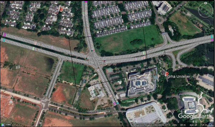
Table 1: Condition data of Foresta BSD intersection approach
| Inter-section Approach | Land User Type | Hazard Class | Road Median | Width (m) | LTOR Phase |
|---|---|---|---|---|---|
| North | Residential | Low | Yes | 16 | Yes |
| East | Commercial | High | Yes | 27 | Yes |
| South | Commercial | High | Yes | 17 | Yes |
| West | Commercial | High | Yes | 27 | Yes |
Table 2: Geometric data of the Foresta BSD intersection
| Intersection Approach | Width (m) | LTOR Phase |
|---|---|---|
| North | 16 | Yes |
| East | 27 | Yes |
| South | 17 | Yes |
| West | 27 | Yes |
Table 3: Traffic volume data of the Foresta BSD intersection
| Inter-section Approach | Motorcycle (veh) | Car (veh) | Truck(veh) | Bus (veh) | Total (Veh) |
|---|---|---|---|---|---|
| North | 938 | 544 | 204 | 0 | 1686 |
| East | 1411 | 1084 | 142 | 4 | 2640 |
| South | 1760 | 274 | 60 | 0 | 2094 |
| West | 2524 | 600 | 102 | 0 | 3226 |
Table 4: Traffic signal of the Foresta BSD intersection (second)
| Inter-section Approach | Red | All Red | Amber | Green | Total | Cycle Time | |
|---|---|---|---|---|---|---|---|
| North | 224 | 5 | 5 | 42 | 276 | 276 | |
| East | 147 | 5 | 5 | 83 | 240 | ||
| South | 110 | 5 | 5 | 51 | 171 | ||
| West | 201 | 5 | 5 | 60 | 271 | ||
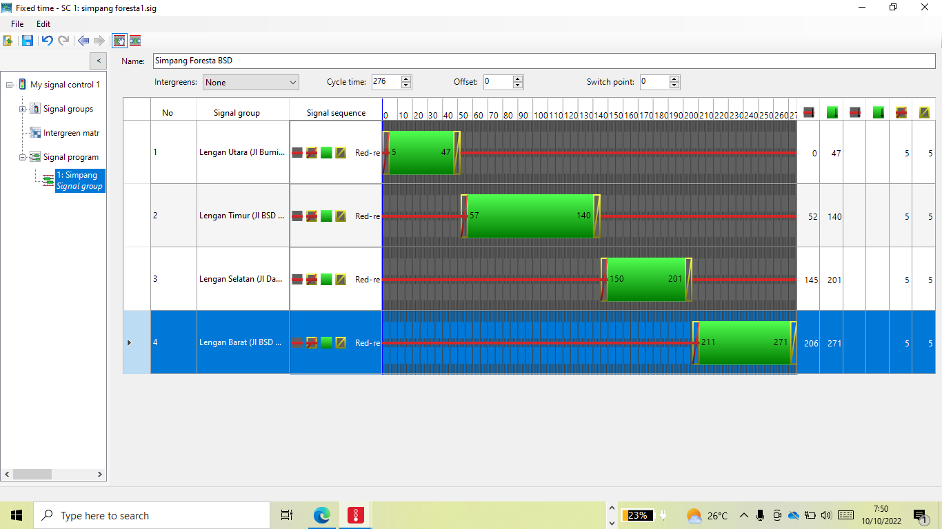
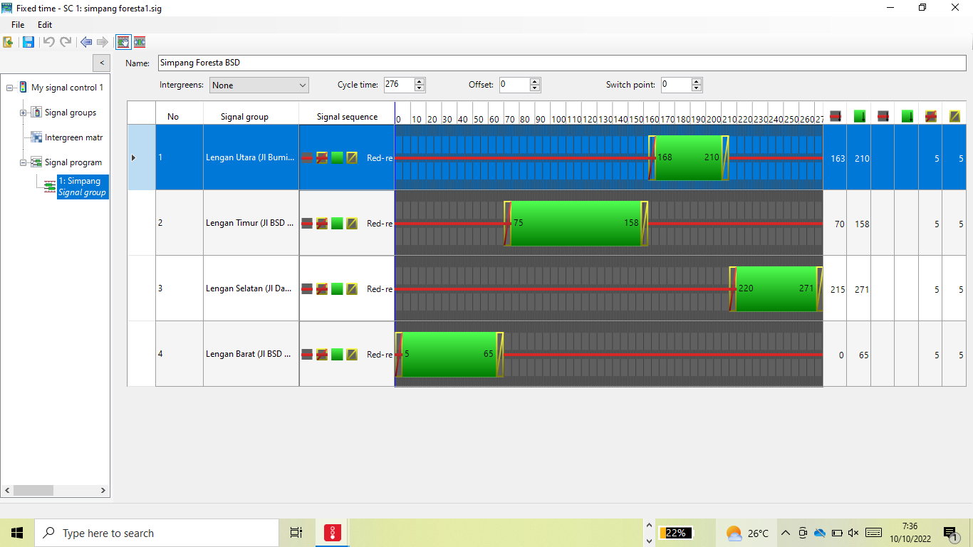
The traffic signal phasing of the Foresta BSD intersection is as follows: North Link (phase 1), East Link (phase 2), South Link (phase 3), and West Link (phase 4). The order of phases can be seen in Figure 5. The cycle times differ slightly across approaches, with relatively long red times and varying green splits. Under the current timing plan, each approach receives a separate green phase, and LTOR movements are permitted. However, given the imbalance in traffic demand, particularly the higher volumes on the east and west approaches, there is potential to improve overall performance by reallocating green time and revising the phase order to better match actual flow patterns. This provides the rationale for the optimisation scenario developed in this study.
4.2. Model Simulation Using PTV Vissim
The collected data is input and processed using PTV Vissim software. After the simulation model is created, it must be calibrated and validated to ensure that it reflects the same conditions as the actual ones. The parameters used in the calibration process are:
a)Driver Behaviour
b)Smoothing Desired Speed Distribution
c)Checking vehicle input position
d)Smoothing and detailing link connectors
The calibration process followed several trial-and-error steps, as summarised in Table 5. The first run (Trial 0) used default parameter values without any adjustments. In subsequent trials, key driver-behaviour parameters were modified to better reflect heterogeneous traffic conditions. For example, the desired position in free flow was changed from “middle of lane” to “any lane” to represent the tendency of drivers in the study area to utilise available lateral space rather than staying strictly in the lane centre. Safety-distance parameters and standstill distances were also reduced to capture the shorter headways typically observed in mixed traffic in Indonesia. In the final trial, vehicle input positions and connector links near the intersection were refined to avoid artificial bottlenecks and to improve the realism of vehicle trajectories.
Table 5: Calibration simulation model
| Trial | Parameter Adjustion | Value | |
|---|---|---|---|
| Before | After | ||
| 0 | First running without any parameter adjustments | - | - |
| 1 | continue from the 1st trial | ||
| Desired position at free flow | Middle of lane | any | |
| Overtake on same lane: on left & right | off | on | |
| 2 | continue from the 1st trial | ||
| Distance standing (at 0 km/h) (m) | 1 | 0.2 | |
| Distance driving (at 50 km/h) (m) | 1 | 0.4 | |
| 3 | continue from the 2nd trial | ||
| Average standstill distance | 2 | 0.6 | |
| The additive part of the safety distance | 2 | 0.6 | |
| Multiplicative part of a safety distance | 3 | 1 | |
| 4 | continue from the 3rd trial | ||
| Checking Vehicle Input in each link | The starting line position of the vehicle input is no longer at the end of the link | Adjustment of the vehicle input starting line position | |
| Connector Link | Connector Link simplified | Each lane near the intersection has its connector link | |
Table 6: Calibration and validation of approach volumes
| Link | Traffic Volume (vehicle) | |||||
|---|---|---|---|---|---|---|
| Existing | Initial Model | 1st Cal | 2nd Cal | 3rd Cal | 4th Cal | |
| North Link | 1.686 | 720 | 804 | 1291 | 1253 | 1281 |
| East Link | 2.640 | 2597 | 2596 | 2595 | 2597 | 2598 |
| South Link | 934 | 1584 | 820 | 905 | 906 | 956 |
| West Link | 3.226 | 790 | 1043 | 2144 | 2168 | 2596 |
The trial-and-error process was carried out based on the survey results collected in the field. For example, in the desired-position parameter under free-flow conditions, the default value in PTV VISSIM is "middle of lane".
However, in the study area, drivers do not always remain in the middle of the lane under free-flow conditions, so the parameter was adjusted to "any lane". After calibration, the model was validated using observed traffic volumes at selected count lines within the coded network. Table 6 reports the observed and simulated traffic volumes at the count lines used for calibration and validation and should be interpreted separately from the class-aggregated approach totals shown in Table 3. The initial calibration results were still far from the observed conditions, so the model was recalibrated iteratively. After the 3rd and 4th calibration trials, the model achieved an R² value of 0.9193, indicating substantially improved agreement between the simulated and observed flows. The results of the R² calculation are shown in Figures 6–9.
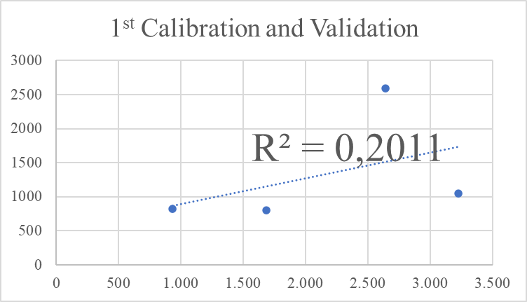
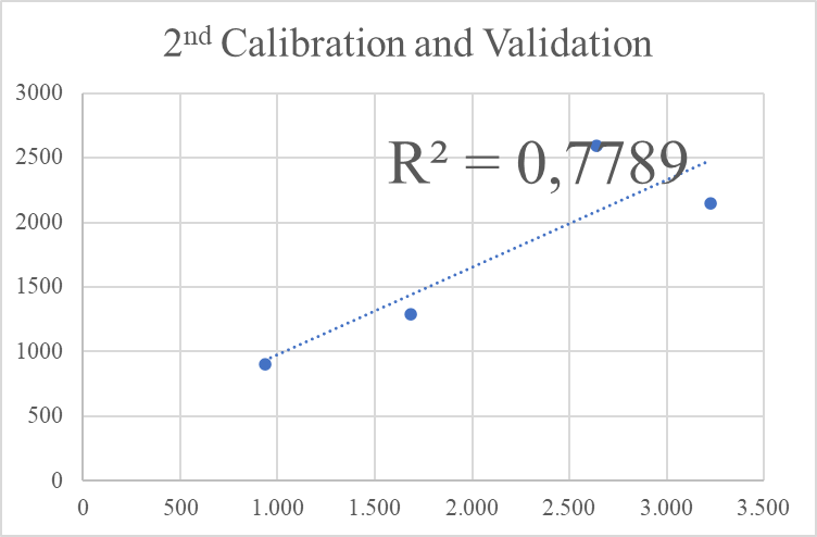
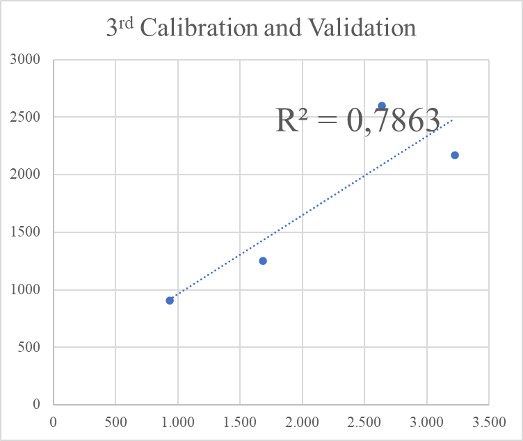
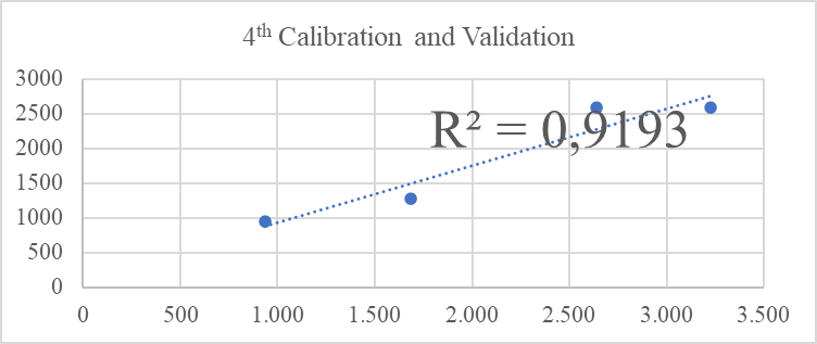
Figures 6–9 show the progressive improvement of the calibration results from Trial 1 to Trial 4. In Figure 6, the scatter points are still widely dispersed from the regression line, indicating that the default and early-adjusted parameters were not yet able to reproduce the observed traffic pattern well. Figure 7 shows a modest improvement after the first behavioural refinements, but noticeable deviations remain, particularly on the heavily loaded approaches. In Figures 8 and 9, the data points move closer to the trend line, and the R² values increase, showing that successive adjustments to safety-distance parameters, vehicle input positions, and connector details improved the match between the simulation and the field data. Trial 4 provides the best overall fit and was therefore used for scenario testing.
4.3. Optimization Scenario
The next stage is applying the optimization scenario. In this research, optimization was carried out by changing the phase sequence of the traffic signal, prioritizing traffic on the West and East lanes, which have higher traffic density during the afternoon rush hour. The change in the phase sequence of the traffic signal is shown in Figure 10.
Network-level performance indicators for the existing condition and the phase-change scenario are presented in Table 7. The results show that implementing the revised phase sequence leads to a reduction in average delay from 246.93 s to 238.35 s, a decrease of about 8.6 s (3.5%). The average stopped delay decreases from 212.48 s to 204.58 s (around 3.7% reduction), and the total number of stops decreases from 51,492 to 48,840, a reduction of 2,652 stops or about 5.2%. Based on standard HCM control-delay categories for signalised intersections, both
scenarios fall within LOS F because the average delay remains above 80 s/veh, although the phase-change scenario still provides measurable operational improvement.
Although the relative reductions in delay may appear modest, they are meaningful in the context of a heavily loaded urban intersection operating under peak-hour conditions. The decrease in the number of stops is significant, as it contributes not only to smoother traffic flow and shorter travel times but also to lower fuel consumption and reduced emissions, as discussed in the next subsection. The results are consistent with previous studies which show that signal-timing optimisation can improve intersection performance under heterogeneous urban traffic.
Overall, however, the net effect of the optimisation scenario is a reduction in total emissions and fuel consumption at the intersection, as summarised in Figure 11. The decrease in average CO, NOx, and VOC emissions and fuel consumption is consistent with the reductions in delay and number of stops reported in Table 7. These findings support previous research indicating that more efficient signal timing can reduce greenhouse gas emissions and improve air quality around urban intersections. At the same time, the results also underline the need to consider both traffic performance and environmental impacts when designing and evaluating signal control strategies.
Table 7: Network performance analysis
| Parameter | Network Performance | |
|---|---|---|
| Existing Condition | Phase Change Scenario Implementation | |
| Delay Average (seconds) | 246,93 | 238,35 |
| Average stopped delay (seconds) | 212,48 | 204,58 |
| Stops (total) | 51492 | 48840 |
| Level of Service (HCM) | F | F |
Table 8: Emission CO
| Link | Emission CO (gram) | |
|---|---|---|
| Existing Condition | Scenario Condition (Phase Change) | |
| Bumi Foresta street (North Link) | 8.215.311 | 8.202.656 |
| BSD Grand Boulevard street (East Link) | 497.603 | 611.327 |
| Damai Foresta street (South Link) | 2.001.179 | 2.001.174 |
| BSD Grand Boulevard street (West Link) | 21.706.335 | 21.492.077 |
Table 9: Emission NOX
| Link | Emission NOX (gram) | |
|---|---|---|
| Existing Condition | Scenario Condition (Phase Change) | |
| Bumi Foresta street (North Link) | 1.598.401 | 1.595.939 |
| BSD Grand Boulevard street (East Link) | 96.816 | 118.942 |
| Damai Foresta street (South Link) | 389.357 | 389.356 |
| BSD Grand Boulevard street (West Link) | 4.223.264 | 4.181.577 |
Table 10: Emission VOC
| Link | Emission VOC (gram) | |
|---|---|---|
| Existing Condition | Scenario Condition (Phase Change) | |
| Bumi Foresta street (North Link) | 1.903.978 | 1.901.045 |
| BSD Grand Boulevard street (East Link) | 115.324 | 141.681 |
| Damai Foresta street (South Link) | 463.793 | 463.791 |
| BSD Grand Boulevard street (West Link) | 5.030.653 | 4.980.996 |
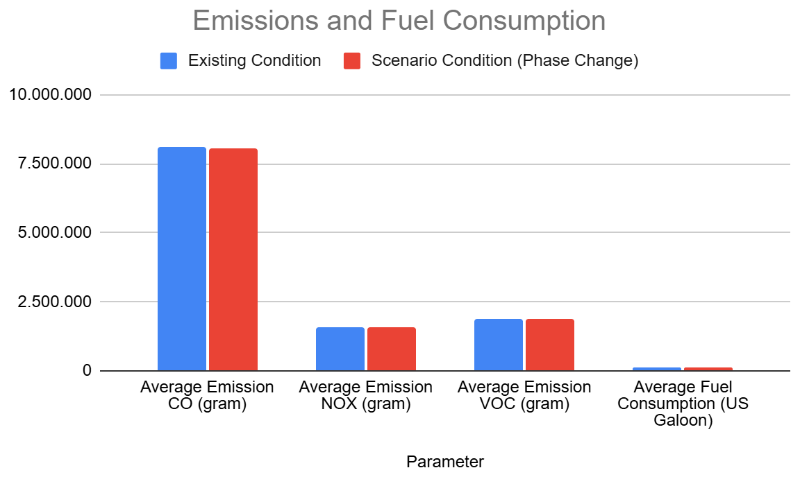
After conducting a comprehensive analysis of travel time, delays, queue length, and travel speed, the phase-change scenario generally performs better than the current condition. Under both the existing and optimised conditions, the intersection still operates at LOS F during the analysed peak hour, which indicates that congestion remains severe even after the timing revision. Nevertheless, the reduction in average delay, stopped delay, and total stops demonstrates that signal phasing adjustments can still generate measurable operational and environmental benefits under existing geometric constraints. In addition, phase changes reduced average CO emissions from 8,105,107 grams to 8,076,809 grams, average NOx emissions from 1,576,960 grams to 1,571,454 grams, average VOC emissions from 1,878,437 grams to 1,871,878 grams, and fuel consumption from 115,953 US gallons to 115,548 US gallons. The present study provides newly structured evidence on signalised-intersection performance improvement by integrating field-measured traffic behaviour, delay diagnostics, and scenario-based optimisation. Unlike previous studies that focus solely on capacity analysis, this research presents a practical, data-driven approach to modifying cycle length, green-time allocation, and phasing schemes to reduce overall delay and improve intersection performance. The findings offer actionable guidance for traffic engineers and local authorities, particularly in prioritising interventions that generate the most significant operational impact under existing geometric constraints.
5. Conclusion
This research was conducted to evaluate the performance of the Foresta BSD Intersection using PTV Vissim. The calibration and validation of the model were carried out by trial and error, considering driver behaviour, traffic volume, and desired speed distribution. This research concludes that it positively impacts intersection performance by conducting optimisation scenarios on phase changes in the traffic signal, such as decreasing the average delay time for each vehicle and reducing the number of stops for cars stuck at the intersection.
After conducting a comprehensive analysis of travel time, delays, queue length, and travel speed, the scenario of phase change organisation in the core area generally performs better than the current condition. Currently, the road network at the Foresta BSD intersection generally serves traffic demand with reasonable efficiency. Traffic management measures and other interventions, such as phase changes, restrictions on excessive vehicle use, and even the addition of lanes at the intersection, are necessary to improve the intersection's performance. Phase changes to improve intersection performance can reduce average delay, stop delay, and total stops. In addition, phase changes can reduce emissions generated by vehicles, including the average CO emissions, which decreased from 8,105,107 grams to 8,076,809 grams; average NOX emissions, which decreased from 1,576,960 grams to 1,571,454 grams; average VOC emissions, which decreased from 1,878,437 grams to 1,871,878 grams; and fuel consumption, which decreased from 115,953 US gallons to 115,548 US gallons.The present study provides newly structured evidence on signalized-intersection performance improvement by integrating field-measured traffic behaviour, delay diagnostics, and scenario-based optimisation. Unlike previous studies that focus solely on capacity analysis, this research present a practical, data-driven approach to modifying cycle length, green-time allocation, and phasing schemes to reduce overall delay and improve intersection level of service. The findings offer actionable guidance for traffic engineers and local authorities, particularly in prioritising interventions that generate the most significant operational impact under existing geometric constraints.
In conclusion, the findings confirm that optimizing signal phasing at the Forerstra BSD intersection provides measurable operational and environmental benefits. The implementation of a phase-change scenario not only improves key traffic performance indicators such as delay, queue length, and travel speed but also contributes to reductions in vehicle emissions and fuel consumption. These results demonstrate that relatively low-cost traffic management strategies, particularly signal timing and phase reorganization, can significantly enhance intersection efficiency without requiring major infrastructure expansion. Therefore, the study highlights the importance of data-driven traffic signal optimization as a practical and sustainable approach for improving urban intersection performance, especially in rapidly growing metropolitan areas where traffic demand continues to increase.
Future research should expand the applicability of the proposed framework by incorporating real-time adaptive signal control, multimodal performance indicators (including pedestrian and public-transport delays), and simulation-based sensitivity testing across different urban corridor typologies. This direction will strengthen the model’s robustness and improve its relevance for broader urban mobility planning.
References
- A.Y. Nurhidayat, H. Widyastuti, Sutikno, D.P. Upahita, and A. Roschyntawati, “Impact of traffic volume on the pollution cost, value of time, and travel time cost in jakarta city centre area,” Civ. Eng. Archit., 11 (5) 3209–3220 (2023). doi:10.13189/cea.2023.110830.
- G. Sugiyanto, “The effect of congestion pricing scheme on the generalized cost and speed of a motorcycle,” Walailak J. Sci. Technol., 15 (1) 95–106 (2018). doi:10.48048/wjst.2018.2347.
- Y. Perez, and F.H. Pereira, “Simulation of traffic light disruptions in street networks,” Phys. A Stat. Mech. Its Appl., 582 126225 (2021). doi:10.1016/j.physa.2021.126225.
- M.M. Bandi, and V. George, “Microsimulation modelling in vissim on short-term and long-term improvements for mangalore city road network,” Transp. Res. Procedia, 48 (2018) 2725–2743 (2020). doi:10.1016/j.trpro.2020.08.243.
- Y. Zhang, and R. Su, “An optimization model and traffic light control scheme for heterogeneous traffic systems,” Transp. Res. Part C Emerg. Technol., 124 (January) 102911 (2021). doi:10.1016/j.trc.2020.102911.
- Supiyono, L. Djakfar, and A. Wicaksono, “Effect of the countdown timer on driver conduct when a yellow flight is displayed at an intersection,” Evergreen, 11 (2) 1148–1156 (2024). doi:10.5109/7183417.
- H. Widyastuti, A.Y. Nurhidayat, A. Soimun, C. Setyarini, N. El Hafizh, and A. Leliana, “Analysis of mode transportation performance and satisfaction level of jenggala commuter line (sidoarjo-mojokerto),” MATEC Web Conf., 181 (2018). doi:10.1051/matecconf/201818103003.
- D.Y.F.C. Hasibuan, and Muchammad Zaenal Muttaqin, “Performance analysis of sibuhuan market intersection, padang lawas regency, north sumatera,” J. Saintis, 21 (01) 53–60 (2021). doi:10.25299/saintis.2021.vol21(01).6507.
- A.Y. Nurhidayat, A. Roschyntawati, S.P. Primadiyanti, D.P. Upahita, and T. Fiantika, “Impact of traffic volume on vehicle operation cost after covid-19 pandemic in dki jakarta,” Evergreen, 11 (3) 2458–2467 (2024). doi:10.5109/7236888.
- Y.N.R. Hendra, R. Pujiwat, M.M.T. Sampetoding, D.P. Utomo, Sucipto, H. Putra, D. Arianto, W.P. Humang, and M.I.A. Saputro, “Traffic congestion management in south tangerang city as an effort to conserve energy in the transportation sector,” Evergreen, 11 (4) 3595–3605 (2024). doi:10.5109/7326992
- A.A.N.A.J. Wikrama, “Signalized intersection performance analysis (case study of teuku umar barat street- gunung salak street),” 15 (1) (2011). https://doi.org/10.37680/almikraj.v5i2.6964 [DOI]
- N. Rorong, L. Elisabeth, and J.E. Waani, “Unsignalized intersection performance analysis,” 3 (11) (2015). https://doi.org/10.52046/jssh.v5i1.2566 [DOI]
- L.L. Di Stasi, F. Angioi, M. Bassani, C. Diaz-Piedra, and A. Megias-Robles, “The effect of traffic light spacing and signal congruency on drivers’ responses at urban intersections,” Transp. Eng., 8 (March) 100113 (2022). doi:10.1016/j.treng.2022.100113.
- Y. Wang, C. Zhang, P. Ji, T. Si, and Z. Zhang, “Effect of pedestrian traffic light on traffic flow accompany with pedestrian crossing,” Physica A, 576 126059 (2021). doi:10.1016/j.physa.2021.126059.
- A.Y. Nurhidayat, A. Utami, and D.P. Upahita, “The impact of congestion pricing on public transport utilization in jakarta, indonesia,” Evergreen, 12 (4) 2058–2069 (2025). doi:10.5109/7402637.
- Y.N.R. Hendra, D.P. Upahita, R. Pujiwat, N. Fitriana, M.I.A. Saputro, A.Y. Nurhidayat, D.P. Utomo, S. Sucipto, H. Putra, D. Arianto, M.N. Putri, M.A. Salsabilla, W.P. Humang, M.M.T. Sampetoding, and Y. Yulianta, “Identifying factors influencing public transportation use for routine and non-routine trip (case study: south tangerang city, indonesia),” Evergreen, 12 (4) 2125–2138 (2025). doi:10.5109/7402642.
- J. McCrea, and S. Moutari, “A hybrid macroscopic-based model for traffic flow in road networks,” Eur. J. Oper. Res., 207 (2) 676–684 (2010). doi:10.1016/j.ejor.2010.05.018.
- J.C. Spall, and D.C. Chin, “Traffic-responsive signal timing for system-wide traffic control,” Transp. Res. Part C Emerg. Technol., 5 (3–4) 153–163 (1997). doi:10.1016/S0968-090X(97)00012-0.
- J. García-Nieto, E. Alba, and A. Carolina Olivera, “Swarm intelligence for traffic light scheduling: application to real urban areas,” Eng. Appl. Artif. Intell., 25 (2) 274–283 (2012). doi:10.1016/j.engappai.2011.04.011.
- K. Gao, Y. Zhang, A. Sadollah, and R. Su, “Optimizing urban traffic light scheduling problem using harmony search with ensemble of local search,” Appl. Soft Comput. J., 48 359–372 (2016). doi:10.1016/j.asoc.2016.07.029.
- G. Sfeir, M. Abou-Zeid, and I. Kaysi, “Multivariate count data models for adoption of new transport modes in an organization-based context,” Transp. Policy, 91 (February) 59–75 (2020). doi:10.1016/j.tranpol.2020.03.014.
- S. Sarjana, H. Fachri, and D. Mustikaningsih, “Leveraging carbon footprint derivatives in challenging the effective implementation of sustainable transportation,” Evergreen, 11 (4) 3684–3692 (2024). doi:10.5109/7326999
- H. Abou-Senna, and E. Radwan, “VISSIM/moves integration to investigate the effect of major key parameters on co2 emissions,” Transp. Res. Part D Transp. Environ., 21 39–46 (2013). doi:10.1016/j.trd.2013.02.003.
- S. Roy, D. Cooper, A. Mucci, B. Sana, M. Chen, J. Castiglione, and G.D. Erhardt, “Why is traffic congestion getting worse? a decomposition of the contributors to growing congestion in san francisco-determining the role of tncs,” Case Stud. Transp. Policy, 8 (4) 1371–1382 (2020). doi:10.1016/j.cstp.2020.09.008.
- D. Chen, J. Ignatius, D. Sun, M. Goh, and S. Zhan, “Impact of congestion pricing schemes on emissions and temporal shift of freight transport,” Transp. Res. Part E Logist. Transp. Rev., 118 (June) 77–105 (2018). doi:10.1016/j.tre.2018.07.006.
- C.K. Tang, “The cost of traffic: evidence from the london congestion charge,” J. Urban Econ., 121 (May 2020) 103302 (2021). doi:10.1016/j.jue.2020.103302.
- K. Wu, Y. Chen, J. Ma, S. Bai, and X. Tang, “Traffic and emissions impact of congestion charging in the central beijing urban area: a simulation analysis,” Transp. Res. Part D Transp. Environ., 51 203–215 (2017). doi:10.1016/j.trd.2016.06.005.
- C. Raux, “The potential for co2 emissions trading in transport: the case of personal vehicles and freight,” Energy Effic., 3 (2) 133–148 (2010). doi:10.1007/s12053-009-9065-7.
- Z.S. Kusharsanto, N. Maninggar, and A. Sucipto, “Electric vehicles ecosystem in indonesia: the readiness of infrastructure, policies, and stakeholders,” Evergreen, 11 (2) 1060–1067 (2024). doi:10.5109/7183402.
- A. Rakowska, K.C. Wong, T. Townsend, K.L. Chan, D. Westerdahl, S. Ng, G. Močnik, L. Drinovec, and Z. Ning, “Impact of traffic volume and composition on the air quality and pedestrian exposure in urban street canyon,” Atmos. Environ., 98 260–270 (2014). doi:10.1016/j.atmosenv.2014.08.073.
- J. Currie, and R. Walker, “Traffic congestion and infant health: evidence from e-zpass,” Am. Econ. J. Appl. Econ., 3 (1) 65–90 (2011). doi:10.1257/app.3.1.65.
- J. Lelieveld, J.S. Evans, M. Fnais, D. Giannadaki, and A. Pozzer, “The contribution of outdoor air pollution sources to premature mortality on a global scale,” Nature, 525 (7569) 367–371 (2015). doi:10.1038/nature15371.
- S.S. Lim, T. Vos, A.D. Flaxman, G. Danaei, K. Shibuya, H. Adair-Rohani, M. Amann, M. Ezzati, et al., “A comparative risk assessment of burden of disease and injury attributable to 67 risk factors and risk factor clusters in 21 regions, 1990-2010: a systematic analysis for the global burden of disease study 2010,” Lancet, 380 (9859) 2224–2260 (2012). doi:10.1016/S0140-6736(12)61766-8.
- C.P. Green, J.S. Heywood, and M. Navarro, “Traffic accidents and the london congestion charge,” J. Public Econ., 133 11–22 (2016). doi:10.1016/j.jpubeco.2015.10.005.
- H. Li, D.J. Graham, and A. Majumdar, “The effects of congestion charging on road traffic casualties: a causal analysis using difference-in-difference estimation,” Accid. Anal. Prev., 49 366–377 (2012). doi:10.1016/j.aap.2012.02.013.
- B.C. Ezell, R. Michael Robinson, P. Foytik, C. Jordan, and D. Flanagan, “Cyber risk to transportation, industrial control systems, and traffic signal controllers,” Environ. Syst. Decis., 33 (4) 508–516 (2013). doi:10.1007/s10669-013-9481-2.
- A. Mhirech, and A. Alaoui-Ismaili, “The effect of traffic light on accident probability in open and periodic boundaries system,” Phys. A Stat. Mech. Its Appl., 434 226–231 (2015). doi:10.1016/j.physa.2015.03.050.
- B.B. Park, and J.D. Schneeberger, “Calibration and validation case study of vissim simulation model for a coordinated actuated signal system,” (03) 185–192 (2003). doi:10.3141/1856-20
- J. Zhao, V.L. Knoop, and M. Wang, “Microscopic traffic modeling inside intersections: interactions between drivers microscopic traffic modeling inside intersections: interactions between drivers,” (July) (2022). doi:10.1287/trsc.2022.1163.This.
- K. Bhattacharyya, B. Maitra, and M. Boltze, “Calibration of micro-simulation model parameters for heterogeneous traffic using mode-specific performance measure,” Transp. Res. Rec., (2020). doi:10.1177/0361198119900130.
- A. Stevanovic, J. Stevanovic, K. Zhang, and S. Batterman, “Optimizing traffic control to reduce fuel consumption and vehicular emissions integrated approach with vissim, cmem, and visgaost,” Transp. Res. Rec. J. Transp. Res. Board, 105–113 (2009). doi:10.3141/2128-11.
- S.H. Kamble, T. V Mathew, and G.K. Sharma, “Development of real-world driving cycle: case study of pune, india,” Transp. Res. Part D, 14 (2) 132–140 (2009). doi:10.1016/j.trd.2008.11.008.
- O.F. Suryaningsih, H. Hermansyah, and E. Kurniati, “Signalized intersection performance analysis (case study hasanuddin street-kamboja street, sumbawa besar),” INERSIALN civil and architecture., 16 (1) 74–84 (2020). doi:10.21831/inersia.v16i1.31317.
- M. Kools, R.A.C. Ruiter, M.W.J. Van De Wiel, and G. Kok, “The effects of headings in information mapping on search speed and evaluation of a brief health education text,” J. Inf. Sci., 34 (6) 833–844 (2008). doi:10.1177/0165551508089719.
- O.Z. Tamin, “Transportation Planning and Modeling,” 2000.
- Z. Zhu, S. Chen, Y. Yang, A. Hu, and X. Zheng, “VISSIM simulation based expressway exit control modes research,” Procedia Eng., 137 738–746 (2016). doi:10.1016/j.proeng.2016.01.311.
- C.M. Weyland, M. V. Baumann, H.S. Buck, and P. Vortisch, “Parameters influencing lane flow distribution on multilane freeways in ptv vissim,” Procedia Comput. Sci., 184 (2019) 453–460 (2021). doi:10.1016/j.procs.2021.03.057.
- E. Nyame-Baafi, C.A. Adams, and K.K. Osei, “Volume warrants for major and minor roads left-turning traffic lanes at unsignalized t-intersections: a case study using vissim modelling,” J. Traffic Transp. Eng. (English Ed., 5 (5) 417–428 (2018). doi:10.1016/j.jtte.2018.01.005.