
Abstract
One crucial aspect of weather forecasting is rainfall prediction, which has a direct impact on agricultural planning and flood risk prevention. Therefore, this study aims to develop a rainfall prediction model by applying a RainAI is a hybrid One-Dimensional Convolutional Neural Network (1D-CNN) - Long Short-Term Memory (LSTM) model along with data preprocessing using K-Nearest Neighbor (KNN) imputation to handle missing values. The model was developed using meteorological datasets collected from Indonesia Meteorology, Climatology, and Geophysics Agency (BMKG). The dataset includes several weather parameters temperature, humidity, wind speed, wind direction, and sunlight duration recorded at daily intervals. In the modeling stage, two deep learning methods are employed: 1D-CNN for spatial feature extraction from time series data, and LSTM for capturing long-term sequential patterns. These are combined into a hybrid model for rainfall prediction. Experimental results using the 1D-CNN-LSTM hybrid model yielded an RMSE of 14.066 mm and MAE of 6.673 mm. Furthermore, testing the model for predicting average weekly rainfall resulted in RMSE of 9.915 mm and MAE of 5.273 mm. Additionally, evaluation of different window sizes showed that using 15 historical data points produced the best performance, with RMSE of 15.142 mm and MAE of 7.942 mm.
Keywords: 1D-CNN, Indonesia, KNN imputation, LSTM, Rainfall prediction
Outline
1. Introduction
Climate refers to the average weather conditions in a particular region over a long period. Weather parameters such as air pressure, rainfall, wind, temperature, and sunlight at specific times and locations contribute to the climatic characteristics of an area. Rainfall is a key component of the climate system that significantly affects various sectors, including agriculture, flood disaster mitigation, and clean water resource management. Currently, rainfall patterns are becoming increasingly unpredictable due to global climate change, posing challenges for multiple sectors1)
Based on data from the period 1961–2010, there has been a 25% increase in extreme rainfall events (>100 mm/day), indicating a rising risk of flooding in urban areas2). Meanwhile, data from the past 40 years (1981–2021) show an average annual rainfall increase of 12.72 mm3). In addition, the number of days with rainfall exceeding 20 mm per day has increased by up to 59 days, while extreme rainfall events above 100 mm per day have risen by 8 days per year. The data also indicate that the cycle of extreme weather events now tends to occur every five years4). Therefore, this study aims to develop an artificial intelligence-based model to predict rainfall.
In developing the rainfall prediction model, data obtained from the Meteorology, Climatology, and Geophysics Agency (BMKG) of Indonesia were used. BMKG is a government agency responsible for providing services related to weather, climate, and geophysical activities such as earthquakes and tsunamis. Established in 1841, the agency continues to support the government in making data-driven decisions5,6). The dataset provided by BMKG served as the basis for model development. However, one of the challenges encountered was the presence of missing values in the data. These missing values were primarily caused by measurement errors or technical issues. To address this problem, a data preprocessing step was conducted using the K-Nearest Neighbor (KNN) imputation method, which fills in missing values based on the patterns or proximity of existing data points7-9).
After the preprocessing stage, the processed dataset (with missing values handled) was used to train the model for rainfall prediction. The choice of modeling method was based on the time-series nature of the data. Therefore, deep learning-based approaches such as One-Dimensional Convolutional Neural Network (1D-CNN) and Long Short-Term Memory (LSTM) were selected. The deep learning modeling process produced three sets of results: first, the model performance using the 1D-CNN method; second, the model performance using the LSTM method; and third, the model performance using a hybrid approach combining 1D-CNN and LSTM. The 1D-CNN was chosen for its effectiveness in extracting spatial features, while LSTM is well-suited for handling sequential data such as time-series10-12).
Previous studies related to weather prediction have demonstrated various strengths, both in terms of the methods applied and the data utilized. Table 1 presents a summary of related research on weather prediction using deep learning models. However, further research involving the development of a rainfall prediction model using BMKG data combined with K-Nearest Neighbor (KNN) imputation to handle missing values, along with a hybrid model integrating 1D-CNN and LSTM, has not yet been explored. This study is expected to provide valuable insights for relevant stakeholders in supporting early mitigation of disaster risks such as floods and droughts through more accurate rainfall prediction.
Table 1: Summary of Related Studies on Weather Prediction
2. Methodology
2.1. System Overview
The research workflow is illustrated in Figure 1. The initial stage of the study begins with a literature review to gather relevant references related to weather prediction based on artificial intelligence. The next stage involves collecting data from weather monitoring stations, where the data obtained has already undergone a validation process, and the measurement instruments used comply with established standards.
The collected weather data initially lacks sufficient quality and requires improvement to achieve optimal model performance. One of the issues encountered in the dataset is the presence of missing values in several data rows. To address this, the KNN imputation technique is applied. KNN imputation works by calculating the distance from the nearest neighboring values to estimate and fill in the missing values18). Another preprocessing step involves converting categorical values into numerical format using encoding techniques.
The dataset that has undergone preprocessing is then split into two parts: training and testing datasets. A larger portion is allocated for training to enhance the model's ability to learn and recognize patterns. The training process employs deep learning methods, namely 1D-CNN and LSTM19,20). The resulting 1D-CNN-LSTM model is then evaluated using RMSE and MAE metrics to assess its performance21).
2.2. Data Description
This study uses weather measurement data collected by the Class I Meteorological Station Ngurah Rai, which operates under the Indonesian Meteorology, Climatology, and Geophysics Agency (BMKG)6). The weather data was gathered from January 1, 2020, to December 24, 2024. According to the dataset, weather measurements were recorded daily, resulting in one data entry per day. Consequently, the dataset contains a total of 1,819 rows of data over the specified period. Table 2 presents a description of the BMKG dataset, which includes ten main attributes that provide information related to weather conditions.
Based on the data description presented in Table 2, the target attribute is rainfall (rr), which represents the daily recorded amount of rainfall measured in millimeters (mm). This attribute is used as the target variable in the prediction modeling process, as the rainfall data is continuous in nature. Meanwhile, other attributes—such as temperature (tn, tx, tavg), humidity (rh_avg), wind speed (ff_x, ff_avg, ddd_x, ddd_car), and sunlight duration (ss) are used as input features. According to the data documentation, a value of 8888 indicates that the data could not be measured, a value of 9999 means the measurement was not conducted,

and a blank (missing) value indicates missing data (NaN), as shown in Table 3.
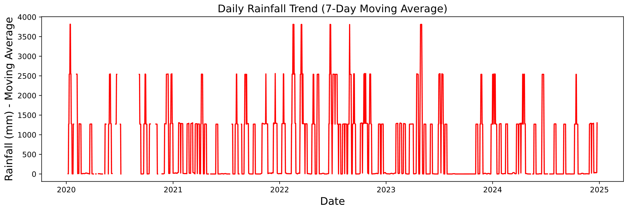
Table 4 presents the descriptive statistics of the dataset, including the minimum, maximum, mean, and standard deviation for all numerical features. The results indicate that the tx attribute contains a maximum value of 9999, which suggests the presence of unmeasured data. Similarly, the rr (rainfall) attribute contains a value of 8888, indicating invalid data. Therefore, these values need to be imputed or replaced. Additionally, the rainfall data (rr) shows a large number of zero values, indicating days without rainfall, as well as several extreme values that cause the data distribution to be skewed. A visualization of the rainfall distribution (rr) is shown in Figure 2. Furthermore, Figure 3(a) illustrates the daily rainfall fluctuation throughout the year, while Figure 3(b) displays the average rainfall fluctuation over a seven-day period.
Table 2: Description of Climate Measurement Data by BMKG
| Atribut | Data Type | Unit | Description |
|---|---|---|---|
| date | date | - | Weather measurement time |
| tn | float | ℃ | Temperature minimum |
| tx | float | ℃ | Temperature maximum |
| tavg | float | ℃ | Temperature avarage |
| rh_avg | integer | % | Humidity average |
| rr | float | mm | Rainfall |
| ff_x | integer | m/s | wind speed |
| ff_avg | integer | m/s | Wind average |
| ddd_x | integer | o | Wind direction at maximum speed |
| ddd_car | varchar | o | Most frequent wind direction |
| ss | float | hour | Duration of sunshine |
Table 3: Climate Measurement Data
| date | tn | tx | tavg | rh_avg | rr | ss | ff_x | ddd_x | ff_avg | ddd_car |
|---|---|---|---|---|---|---|---|---|---|---|
| 05-01-2020 | 25.6 | 31.3 | 28.6 | 81 | 8.1 | Nan | 8 | 260 | 6 | W |
| 09-01-2020 | 26.8 | 31.2 | 28.7 | 76 | 8888 | 8.5 | 9 | 300 | 4 | W |
| 10-01-2020 | 26.5 | 31 | 28.7 | 72 | 0 | Nan | 6 | 260 | 4 | W |
| 11-01-2020 | 27 | 31.4 | 27.9 | 82 | 8888 | 12.3 | 9 | 280 | 6 | W |
| 14-03-2021 | 24.5 | 9999 | 27.8 | 80 | 3.5 | 9.7 | 5 | 280 | 3 | N |
| 25-05-2021 | 26.6 | 30.8 | Nan | Nan | 0 | 9 | 5 | 110 | 3 | E |
| 23-10-2022 | 24.4 | 31.1 | 27.7 | 83 | 8888 | 6.2 | 6 | 300 | 3 | W |
| 09-07-2023 | 26 | 28.8 | 26.9 | 87 | 8888 | 2.5 | 7 | 100 | 4 | E |
| 07-06-2024 | Nan | Nan | Nan | 84 | 0 | 9.8 | 5 | 120 | 3 | SE |
| … | … | … | … | … | … | … | … | … | … | … |
| 30-11-2024 | 26 | 30.8 | 27.6 | 87 | 48.6 | 5.8 | 7 | 300 | 4 | W |
Table 4: Descriptive Statistics of the Dataset
| tn | tx | tavg | rh_avg | rr | ss | ff_x | ddd_x | ff_avg | |
|---|---|---|---|---|---|---|---|---|---|
| count | 1776 | 1803 | 1786 | 1787 | 1786 | 1797 | 1819 | 1762 | 1819 |
| mean | 25.1 | 36.12 | 27.58 | 80.97 | 702.63 | 7.66 | 5.97 | 176.63 | 3.33 |
| std | 1.13 | 234.8 | 0.99 | 4.28 | 2387.91 | 3.03 | 1.85 | 78.58 | 1.33 |
| min | 20.2 | 26.8 | 24.2 | 64 | 0 | 0 | 3 | 10 | 1 |
| 25% | 24.4 | 29.7 | 26.9 | 78 | 0 | 6.2 | 5 | 110 | 2 |
| 50% | 25.2 | 30.6 | 27.6 | 81 | 0 | 8.3 | 6 | 130 | 3 |
| 75% | 25.8 | 31.4 | 28.3 | 84 | 8.38 | 10.1 | 7 | 260 | 4 |
| max | 28.2 | 9999 | 30.3 | 97 | 8888 | 13 | 20 | 360 | 12 |


2.3. Study Area
The study location uses meteorological observation data obtained from the Class I Meteorological Station Ngurah Rai operated by BMKG, which is located in Badung Regency, Bali Province, Indonesia, at coordinates -8.742928483323352, 115.16428944907665. Bali Island is a tropical region whose weather conditions are strongly influenced by the monsoon system, seasonal wind patterns, and interactions between the atmosphere and the ocean22). In general, the rainfall pattern in Bali is divided into two main seasons, namely the wet season, which usually occurs from November to March, and the dry season, which takes place from April to October. However, rainfall patterns in recent years have shown increasingly dynamic changes due to climate phenomena such as El Nino Southern Oscillation (ENSO), Indian Ocean Dipole (IOD), as well as the impacts of global climate change23,24).
The Class I Meteorological Station Ngurah Rai has an important role because it represents tropical coastal weather conditions in southern Bali. The southern Bali region is a center of high economic activity, a major tourist destination, and is highly vulnerable to flooding conditions. Therefore, rainfall prediction is important for water resource management, policy planning, and disaster mitigation. This geographical context supports the importance of developing a deep learning-based rainfall prediction model by utilizing direct data from meteorological station observations.
2.4. Preprocessing Data
This section describes the preprocessing steps carried out to address the issue of attributes containing values of 8888 and 9999. These values were replaced with null to facilitate the identification of missing data. After replacing them with null values, missing data were found in several key attributes: 43 in tn, 17 in tx, 33 in tavg, 32 in rh_avg, 173 in rr, 22 in ss, and 57 in ddd_x, as shown in Figure 4.
Next, the missing values were handled using the KNN imputation method. This method fills in missing (null) values by calculating the distance between data points using the Euclidean Distance metric (Equation 1), and then replacing the missing values with the average of the nearest (k) neighbors. In Equation 1, represents the Euclidean distance between two points and , where is the i-th attribute of point , is the i-th attribute of point , and is the total number of attributes7,25,26).
Figure 5 shows the results of the imputation process. Figure 5(a) displays the data before imputation, while Figure 5(b) shows the data after the missing values have been filled.
The next step involved converting categorical data into numerical format. The ddd_car attribute, which indicates wind direction and is categorical in nature, was transformed using encoding by mapping each category to a numeric value as follows: 'C': 0, 'E': 1, 'N': 2, 'NE': 3, 'NW': 4, 'S': 5, 'SE': 6, 'SW': 7, 'W': 8, as illustrated in Figure 6.
To determine the relationship between the target attribute (rr) and other attributes, a correlation calculation was performed using Equation 2, resulting in a correlation matrix as shown in Table 4. In Equation 2, r represents the correlation coefficient between variables, is the value of variable , is the value of variable , and is the number of observations27).
The correlation matrix values in Table 5 show that the target attribute (rr) has a strong relationship with the humidity attribute (rh_avg), with a correlation coefficient of 0.42. It also shows correlations with wind speed (ff_x) and wind direction (ddd_x), with values of 0.17 and 0.3, respectively. Table 6 presents the descriptive statistics of the dataset after preprocessing, indicating that a total of 10 attributes were used in the modeling process.
Next, in the modeling stage, the numerical data having different value ranges were normalized to a common scale to ensure that each feature contributed equally during modeling. This was done using the Min-Max Scaling technique, which transforms values to a range between 0 and 1.

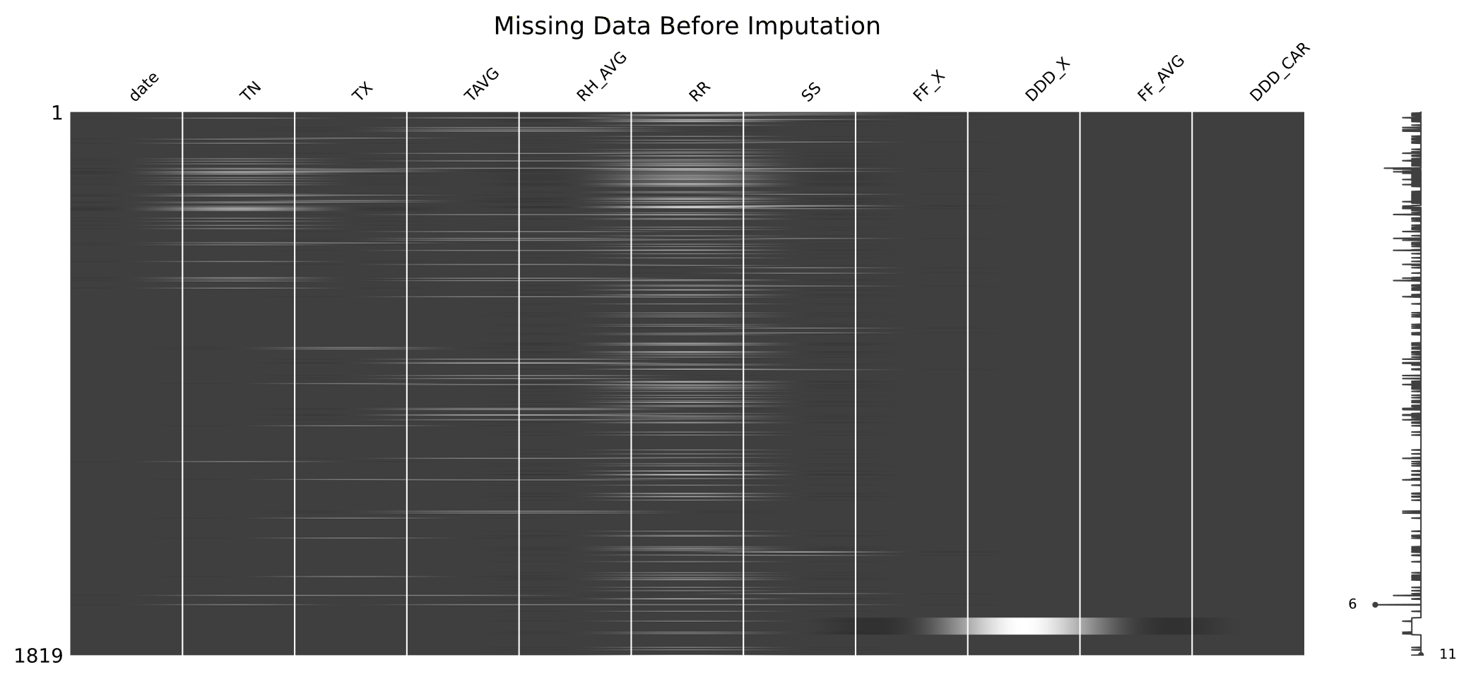


Table 5: Dataset Correlation Coefficient Matrix
| tn | tx | tavg | rh_avg | rr | ss | ff_x | ddd_x | ff_avg | ddd_car | |
|---|---|---|---|---|---|---|---|---|---|---|
| tn | 1 | 0.37 | 0.66 | -0.14 | -0.25 | 0.11 | 0.033 | 0.034 | 0.089 | -0.003 |
| tx | 0.37 | 1 | 0.78 | -0.15 | -0.13 | 0.082 | -0.17 | 0.19 | -0.26 | -0.021 |
| tavg | 0.66 | 0.78 | 1 | -0.25 | -0.18 | 0.086 | -0.057 | 0.18 | -0.036 | 0.05 |
| rh_avg | -0.14 | -0.15 | -0.25 | 1 | 0.42 | -0.31 | 0.067 | 0.23 | -0.057 | 0.056 |
| rr | -0.24 | -0.13 | -0.18 | 0.42 | 1 | -0.36 | 0.17 | 0.31 | 0.09 | 0.16 |
| ss | 0.11 | 0.082 | 0.085 | -0.31 | -0.36 | 1 | -0.13 | -0.29 | -0.055 | -0.13 |
| ff_x | 0.033 | -0.17 | -0.057 | 0.068 | 0.17 | -0.13 | 1 | 0.26 | 0.76 | 0.3 |
| ddd_x | 0.034 | 0.19 | 0.18 | 0.23 | 0.31 | -0.29 | 0.26 | 1 | 0.091 | 0.5 |
| ff_avg | 0.089 | -0.26 | -0.036 | -0.057 | 0.09 | -0.055 | 0.76 | 0.091 | 1 | 0.23 |
| ddd_car | -0.003 | -0.021 | 0.05 | 0.056 | 0.16 | -0.13 | 0.3 | 0.5 | 0.23 | 1 |
Table 6: Descriptive Statistics of the Dataset After Preprocessing
| Atribute | Count | Min | 25% | 50% | 75% | Max | Mean | Std |
|---|---|---|---|---|---|---|---|---|
| tn | 1819 | 20.2 | 24.5 | 25.2 | 25.8 | 28.2 | 25.1 | 1.1 |
| tx | 1819 | 26.8 | 29.8 | 30.6 | 31.4 | 35.1 | 30.5 | 1.1 |
| tavg | 1819 | 24.2 | 26.9 | 27.6 | 28.3 | 30.3 | 27.5 | 0.9 |
| rh_avg | 1819 | 64 | 78 | 81 | 84 | 97 | 80.9 | 4.3 |
| rr | 1819 | 0 | 0 | 0 | 4.1 | 177.4 | 6.1 | 14.9 |
| ss | 1819 | 0 | 6.2 | 8.3 | 10 | 13.0 | 7.6 | 3.0 |
| ff_x | 1819 | 3 | 5 | 6 | 7 | 20 | 5.9 | 1.8 |
| ddd_x | 1819 | 10 | 110 | 130 | 260 | 360 | 176.4 | 77.8 |
| ff_avg | 1819 | 1 | 2 | 3 | 4 | 12 | 3.3 | 1.3 |
| ddd_car | 1819 | 0 | 2 | 8 | 11 | 11 | 7.1 | 3.5 |
2.5. One-Dimensional Convolution Neural Network
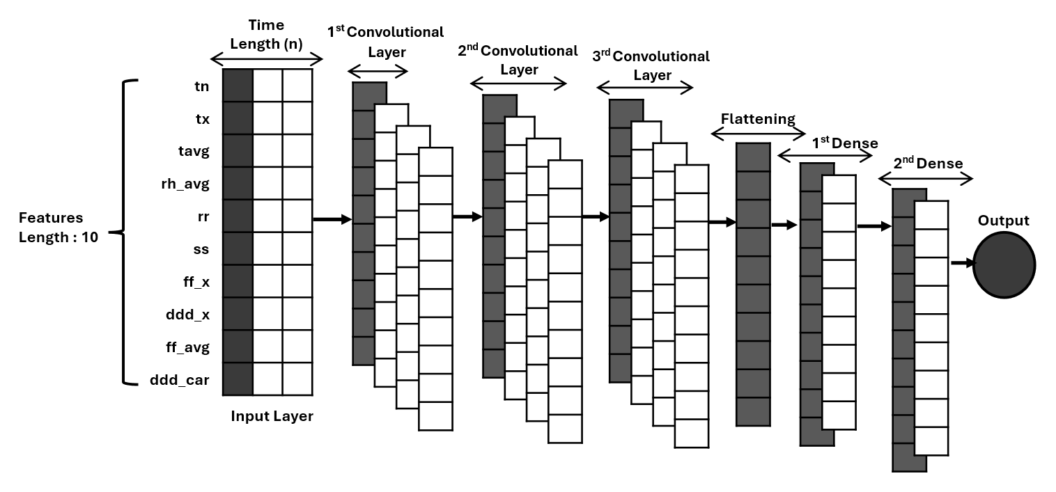
The One-Dimensional Convolution Neural Network (1D-CNN) is used to build a rainfall prediction model, with its architecture illustrated in Figure 7. The model uses 10 input attributes: tn, tx, tavg, rh_avg, rr, ss, ff_x, ddd_x, ff_avg, and ddd_car. These input features form a matrix with dimensions [n, 10], where n represents the time length. Three convolutional layers are applied sequentially, each functioning to extract patterns from the data using filters (kernels). A flattening layer is then used to convert the multidimensional data into a one-dimensional format. Finally, two dense layers are employed to combine the extracted information and produce the final output28,29).
2.6. Long Short-Term Memory (LSTM)

Figure 8 shows the block diagram of an LSTM, which generally consists of three main gates: the input gate, forget gate, and output gate30,31). The equations associated with this diagram are presented in Equations 3–10. In these equations, represents the forget gate value, > is the input gate value, and is the output gate value. Furthermore, denotes the previous hidden state, is the current input, refers to the weights, is the bias, is the candidate value, and represents the cell state12,32).
2.7. 1DCNN - LSTM
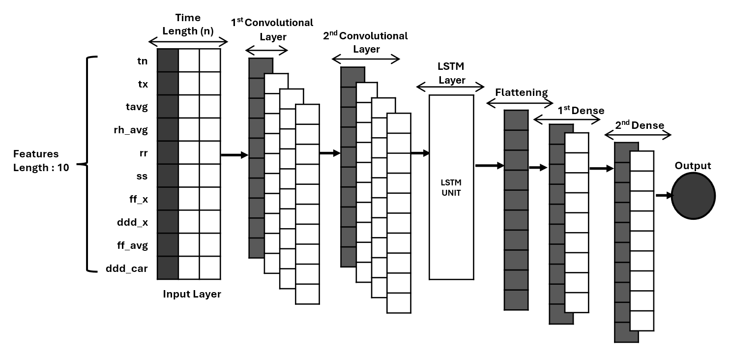
The rainfall prediction model was further enhanced by combining the 1D-CNN and LSTM methods to improve overall performance33-35). Figure 9 illustrates the architecture used for this hybrid model. The model receives 10 input features, which are first passed through a 1D Convolutional layer (1D-CNN) responsible for extracting features and detecting patterns from the data. The output is then forwarded to an LSTM layer, which models temporal relationships in the data over time and identifies sequential patterns using memory units. The output from the LSTM is flattened into a one-dimensional vector through a flattening layer. Finally, a Dense layer is
Table 7: Hyperparameters and Experimental Settings
| Parameter | Value |
|---|---|
| Optimizer | Adam |
| Loss Function | Mean Squared Error (MSE) |
| Evaluation Metrics | RMSE, MAE |
| Number of Epochs | 300 |
| Batch Size | 32 |
| Training-Testing Split | 90% : 10% |
| Input Window Size | 6-16 historical steps |
| Forecast Horizon | 1-step ahead |
| Feature Scaling | Min-Max Normalization |
| Missing Value Treatment | KNN Imputation (k = 3) |
| Data Shuffling | Enabled |
used to integrate the extracted key features and produce the final prediction output.
2.8. Experimental Setup and Hyperparameters
Table 7 presents the hyperparameters and experimental settings used in developing the RainAI. The Adam optimizer was applied to update model weights efficiently during training, while Mean Squared Error (MSE) was used as the loss function. Model performance was evaluated using Root Mean Square Error (RMSE) and Mean Absolute Error (MAE). The training process was conducted for 300 epochs with a batch size of 32. The dataset was divided into 90% training data and 10% testing data. Input sequences used 6-16 historical time steps to predict one future rainfall value (1-step ahead). In addition, Min-Max Normalization was applied for feature scaling, missing values were handled using KNN Imputation with k=3, and data shuffling was enabled to improve training generalization.
All experiments were conducted using Python 3.10 and TensorFlow 2.x in the Google Colab environment. The training process utilized NVIDIA Tesla T4 GPU acceleration with 16 GB RAM to improve computational efficiency.
2.9. Model Performance Evaluation Techniques
The model evaluation process employs several techniques, including Root Mean Square Error (RMSE) to measure the average of error between predicted and actual values, as shown in Equation 11. Mean Absolute Error (MAE) is also used to calculate the average of the absolute differences between predicted and actual values, as presented in Equation 12. The variables in each equation are defined as follows: n is the number of observed data points, is the actual value, and is the predicted value36-39).
3. Result and Discussion
This section presents the testing results from the modeling process, which is divided into several parts to identify the best model configuration. The first testing phase involved adjusting the number of neurons in each hidden layer. Three methods were evaluated: the 1D-CNN method, the LSTM method, and a hybrid method combining 1D-CNN and LSTM. The 1D-CNN and LSTM models each used three hidden layers, while the hybrid model used two layers in the 1D-CNN section and two layers in the LSTM section. The number of neurons in each layer varied, ranging from 8 to 256.
The testing results show that the 1D-CNN model achieved an RMSE value of 14.536 mm, as presented in Table 8 and Figure 10(a). Figure 10(b) displays a comparison between actual and predicted values, with an RMSE of 14.623 mm. For the LSTM model, the obtained RMSE was 14.510 mm, as shown in Table 9 and Figure 11(a), while Figure 11(b) presents the comparison between actual and predicted values with an RMSE of 14.825 mm. Meanwhile, the hybrid model combining 1D-CNN and LSTM produced the most optimal results, with an RMSE of 14.066 mm, as shown in Table 10 and Figure 12(a), and Figure 12(b) presents a comparison with an RMSE of 14.395 mm.
Table 8: 1D-CNN Model Performance with Different Numbers of Neurons
| 1DCNN-1 Neurons | 1DCNN -2 Neurons | 1DCNN -3 Neurons | Dense-1 Neurons | RMSE | MEA |
|---|---|---|---|---|---|
| 32 | 16 | 8 | 8 | 14.631 | 6.833 |
| 64 | 32 | 16 | 8 | 15.036 | 6.126 |
| 64 | 32 | 16 | 16 | 14.956 | 6.429 |
| 64 | 64 | 32 | 16 | 14.833 | 6.662 |
| 128 | 64 | 32 | 16 | 14.732 | 6.848 |
| 128 | 64 | 32 | 32 | 14.629 | 7.043 |
| 128 | 128 | 64 | 32 | 14.623 | 6.362 |
| 150 | 100 | 50 | 10 | 14.795 | 6.848 |
| 150 | 75 | 50 | 20 | 14.650 | 7.252 |
| 150 | 100 | 75 | 32 | 14.647 | 6.025 |
| 200 | 100 | 50 | 32 | 14.536 | 7.757 |
| 200 | 150 | 100 | 64 | 14.732 | 6.534 |
| 250 | 150 | 100 | 64 | 15.025 | 6.032 |
| 256 | 128 | 64 | 64 | 14.987 | 5.839 |
| 256 | 256 | 128 | 128 | 15.109 | 6.514 |


Table 9: LSTM Model Performance with Different Numbers of Neuronss
| LSTM-1 Neurons | LSTM -2 Neurons | LSTM-3 Neurons | Dense-1 Neurons | RMSE | MEA |
|---|---|---|---|---|---|
| 32 | 16 | 8 | 8 | 14.510 | 7.112 |
| 64 | 32 | 16 | 8 | 14.825 | 6.472 |
| 64 | 32 | 16 | 16 | 15.039 | 6.910 |
| 64 | 64 | 32 | 16 | 15.054 | 6.191 |
| 128 | 64 | 32 | 16 | 15.076 | 6.243 |
| 128 | 64 | 32 | 32 | 15.214 | 6.721 |
| 128 | 128 | 64 | 32 | 14.928 | 7.115 |
| 150 | 100 | 50 | 10 | 15.101 | 6.724 |
| 150 | 75 | 50 | 20 | 15.358 | 6.906 |
| 150 | 100 | 75 | 32 | 14.510 | 6.183 |
| 200 | 100 | 50 | 32 | 14.910 | 6.490 |
| 200 | 150 | 100 | 64 | 15.376 | 6.429 |
| 250 | 150 | 100 | 64 | 15.832 | 7.099 |
| 256 | 128 | 64 | 64 | 15.354 | 6.763 |
| 256 | 256 | 128 | 128 | 15.895 | 7.699 |


Table 10: 1DCNN-LSTM Model Performance with Different Numbers of Neurons
| 1DCNN-1 Neurons | 1DCNN -2 Neurons | LSTM-1 Neurons | LSTM-1 Neurons | Dense-1 Neurons | RMSE | MEA |
|---|---|---|---|---|---|---|
| 32 | 16 | 8 | 4 | 8 | 14.981 | 8.171 |
| 64 | 32 | 16 | 8 | 8 | 14.804 | 7.608 |
| 64 | 32 | 16 | 8 | 16 | 14.535 | 7.061 |
| 64 | 64 | 32 | 16 | 16 | 14.750 | 7.531 |
| 128 | 64 | 32 | 16 | 16 | 14.555 | 7.332 |
| 128 | 64 | 32 | 16 | 32 | 14.752 | 7.251 |
| 128 | 128 | 64 | 32 | 32 | 14.789 | 7.226 |
| 150 | 100 | 50 | 25 | 10 | 14.822 | 6.729 |
| 150 | 75 | 50 | 25 | 20 | 14.772 | 7.320 |
| 150 | 100 | 75 | 37 | 32 | 14.942 | 5.923 |
| 200 | 100 | 50 | 25 | 32 | 14.066 | 6.673 |
| 200 | 150 | 100 | 50 | 64 | 14.395 | 6.839 |
| 250 | 150 | 100 | 50 | 64 | 14.784 | 6.087 |
| 256 | 128 | 64 | 32 | 64 | 14.869 | 7.943 |
| 256 | 256 | 128 | 64 | 128 | 14.740 | 7.629 |


RMSE = 14.066, (b) RMSE = 14.395
The second test was conducted using seven-day average data to predict weekly average rainfall. The method used was a combination of 1D-CNN and LSTM, each consisting of two layers. The best results were achieved with an RMSE of 9.915 mm and an MAE of 5.273 mm. The model architecture comprised two 1D-CNN layers, two LSTM layers, and one dense layer, with the number of neurons set to 128, 128, 64, 32, and 32, respectively. The complete test results are presented in Table 11, while Figures 13(a) and 13(b) show the comparison between actual and predicted values, with RMSE values of 9.915 mm and 9.922 mm.
The next testing phase involved selecting the number of previous data points used to predict future values, a parameter known as the window size. In this test, the window size was varied from 6 to 16, meaning the model used between 6 and 16 past data points to predict one future value. Since the data was recorded at daily intervals, a window size of 6 indicates that the model uses the last six days of data to predict the value for the next day. The test results based on different window sizes are presented in Table 12. The results show that a window size of 15 yielded the best model performance, with an RMSE of 15.142 mm and an MAE of 7.942 mm.
Table 11: 1D-CNN–LSTM Model Performance on 7-Day Mean Data
| 1DCNN-1 Neurons | 1DCNN -2 Neurons | LSTM-1 Neurons | LSTM-1 Neurons | Dense-1 Neurons | RMSE | MEA |
|---|---|---|---|---|---|---|
| 32 | 16 | 8 | 4 | 8 | 9.937 | 5.304 |
| 64 | 32 | 16 | 8 | 8 | 9.927 | 5.292 |
| 64 | 32 | 16 | 8 | 16 | 9.938 | 5.306 |
| 64 | 64 | 32 | 16 | 16 | 9.922 | 5.283 |
| 128 | 64 | 32 | 16 | 16 | 9.936 | 5.302 |
| 128 | 64 | 32 | 16 | 32 | 9.935 | 5.301 |
| 128 | 128 | 64 | 32 | 32 | 9.915 | 5.273 |
| 150 | 100 | 50 | 25 | 10 | 9.934 | 5.300 |
| 150 | 75 | 50 | 25 | 20 | 9.931 | 5.295 |
| 150 | 100 | 75 | 37 | 32 | 9.934 | 5.300 |
| 200 | 100 | 50 | 25 | 32 | 9.936 | 5.303 |
| 200 | 150 | 100 | 50 | 64 | 9.931 | 5.295 |
| 250 | 150 | 100 | 50 | 64 | 9.930 | 5.293 |
| 256 | 128 | 64 | 32 | 64 | 9.929 | 5.293 |
| 256 | 256 | 128 | 64 | 128 | 9.930 | 5.294 |


Table 12: Result of Selection Window Size
| Window Size | RMSE | MEA |
|---|---|---|
| 6 | 16.130 | 6.672 |
| 7 | 15.410 | 8.347 |
| 8 | 15.285 | 8.357 |
| 9 | 15.266 | 8.297 |
| 10 | 15.168 | 8.064 |
| 11 | 15.265 | 8.266 |
| 12 | 15.240 | 8.239 |
| 13 | 15.192 | 7.996 |
| 14 | 15.385 | 8.300 |
| 15 | 15.142 | 7.942 |
| 16 | 15.242 | 7.936 |
4. Conclusions
This study developed a rainfall prediction model using 1D-CNN and LSTM methods. The dataset used was weather data from BMKG, recorded daily from 2020 to 2024. The data consisted of 11 weather attributes, including temperature, humidity, wind speed, wind direction, and sunlight duration. Prior to modeling, a preprocessing phase was conducted to handle missing values using KNN imputation and to convert categorical data into numerical format using encoding techniques. Modeling was carried out using three different architectures: 1D-CNN, LSTM, and a hybrid 1D-CNN–LSTM, each comprising three hidden layers with the number of neurons ranging from 8 to 256. The test results showed that the hybrid 1D-CNN–LSTM model achieved the best performance with an RMSE of 14.066 mm and an MAE of 6.673 mm. Further testing using seven-day average data to predict weekly average rainfall yielded an RMSE of 9.915 mm and an MAE of 5.273 mm. In addition, testing different window sizes found that using 15 historical data points produced the highest accuracy, with an RMSE of 15.142 mm and an MAE of 7.942 mm.
Acknowledgements
This work was partly supported by the Research and Community Service Program (PDP), Ministry of Higher Education, Science, and Technology of the Republic of Indonesia, under Grant No. Ref: 129/C3/DT.05.00/PL/2025.
Appendix
The dataset used in this study was obtained from the official portal of Indonesia Meteorology, Climatology, and Geophysics Agency: https://dataonline.bmkg.go.id using observations from the Class I Meteorological Station Ngurah Rai, Badung, Bali. The data cover the period from January 1, 2020, to December 24, 2024, with daily observation frequency, resulting in 1,819 records.
References
- Q. Fu, D. Niu, Z. Zang, J. Huang, and L. Diao, “Multi-Stations’ Weather Prediction Based on Hybrid Model Using 1D CNN and Bi-LSTM,” in: 2019 Chinese Control Conf., 3771–3775 (2019). doi:10.23919/ChiCC.2019.8866496.
- S. Siswanto, G.J. van Oldenborgh, G. van der Schrier, R. Jilderda, and B. van den Hurk, “Temperature, extreme precipitation, and diurnal rainfall changes in the urbanized jakarta city during the past 130 years,” Int. J. Climatol., 36 (9) 3207–3225 (2016). doi:10.1002/joc.4548.
- G.G. Sudarman, T.W. Hadi, N.S. Ningsih, A. Sopaheluwakan, M.R. Syahputra, and F. Marpaung, “Nonstationary changes in annual rainfall over indonesia’s maritime continent,” Adv. Meteorol., 2024 (2024). doi:10.1155/2024/9392844.
- “Annual rainfall change rate analysis,” (2025). https://www.bmkg.go.id/ (accessed June 9, 2025).
- H. Kausarian, J.T.S. Sumantyo, Batara, A. Suryadi, and T. Pangestu, “SAR sentinel data analysis: hydrological dynamics and rainfall patterns in the kampar river basin (2018-2023),” Evergreen, 11 (3) 1558–1567 (2024). doi:10.5109/7236811.
- Indonesian Agency for Meteorology, Climatology, and Geophysics (BMKG), “Meteorology, Climatology, and Geophysics Agency,” n.d. https://www.bmkg.go.id.
- C. Wang, B. Ren, X. Li, and L. Chen, “A CNN-BiLSTM and KNN based missing data imputation for wind power generation forecasting,” in: 2023 IEEE 6th Int. Electr. Energy Conf., 4065–4070 (2023). doi:10.1109/CIEEC58067.2023.10166993.
- B. Setya, R.A. Nurhidayatullah, M.B. Hewen, and K. Kusrini, “Comparative Analysis Of Rainfall Value Prediction In Semarang Using Linear And K-Nearest Neighbor Algorithms,” in: 2023 5th Int. Conf. Cybern. Intell. Syst., 1–5 (2023). doi:10.1109/ICORIS60118.2023.10352274.
- D.M.P. Murti, U. Pujianto, A.P. Wibawa, and M.I. Akbar, “K-Nearest Neighbor (K-NN) based Missing Data Imputation,” in: 2019 5th Int. Conf. Sci. Inf. Technol., 83–88 (2019). doi:10.1109/ICSITech46713.2019.8987530.
- N. Vakitbilir, A. Hilal, and C. Direko\uglu, “Prediction of Daily Solar Irradiation Using CNN and LSTM Networks,” in: R.A. Aliev, J. Kacprzyk, W. Pedrycz, M. Jamshidi, M. Babanli, F.M. Sadikoglu (Eds.), 14th Int. Conf. Theory Appl. Fuzzy Syst. Soft Comput. -- ICAFS-2020, Springer International Publishing, Cham, 230–238 (2021). doi:10.1007/978-3-030-64058-3_28.
- J. Altamirano-Astorga, J.O. Gutierrez-Garcia, and E. Roman-Rangel, “Forecasting indoor air quality in mexico city using deep learning architectures,” Atmosphere (Basel)., 15 (12) (2024). doi:10.3390/atmos15121529.
- I.K.A.A. Aryanto, D. Maneetham, and P.N. Crisnapati, “Enhancing neonatal incubator energy management and monitoring through iot-enabled cnn-lstm combination predictive model,” Appl. Sci., 13 (23) (2023). doi:10.3390/app132312953.
- R. Nagaraj, and L.S. Kumar, “Univariate deep learning models for prediction of daily average temperature and relative humidity: the case study of chennai, india,” J. Earth Syst. Sci., 132 (3) 100 (2023). doi:10.1007/s12040-023-02122-0.
- Q. Guo, Z. He, Z. Wang, S. Qiao, J. Zhu, and J. Chen, “A performance comparison study on climate prediction in weifang city using different deep learning models,” Water, 16 (19) (2024). doi:10.3390/w16192870.
- Q. Guo, Z. He, and Z. Wang, “Monthly climate prediction using deep convolutional neural network and long short-term memory,” Sci. Rep., 14 (1) 17748 (2024). doi:10.1038/s41598-024-68906-6.
- F. Di Nunno, and F. Granata, “Advanced monthly rainfall forecasting in southern lazio: integrating climatic indices, classical or deep neural networks, and a feature selection algorithm,” Water Cycle, (2024). doi:10.1016/j.watcyc.2024.11.005.
- M. Waqas, U.W. Humphries, P.T. Hlaing, A. Wangwongchai, and P. Dechpichai, “Advancements in daily precipitation forecasting: a deep dive into daily precipitation forecasting hybrid methods in the tropical climate of thailand,” MethodsX, 12 102757 (2024). doi:10.1016/j.mex.2024.102757.
- A.K. Tripathi, H. Saini, and G. Rathee, “Missing Values Imputation in Food Consumption: An Analytical Study,” in: 2021 6th Int. Conf. Signal Process. Comput. Control, 303–307 (2021). doi:10.1109/ISPCC53510.2021.9609371.
- N. Madhukumar, E. Wang, Y.-F. Zhang, and W. Xiang, “Consensus forecast of rainfall using hybrid climate learning model,” IEEE Internet Things J., 8 (9) 7270–7278 (2021). doi:10.1109/JIOT.2020.3040736.
- Y. Essa, H.G.P. Hunt, M. Gijben, and R. Ajoodha, “Deep learning prediction of thunderstorm severity using remote sensing weather data,” IEEE J. Sel. Top. Appl. Earth Obs. Remote Sens., 15 4004–4013 (2022). doi:10.1109/JSTARS.2022.3172785.
- I.N.K. Wardana, J.W. Gardner, and S.A. Fahmy, “Estimation of missing air pollutant data using a spatiotemporal convolutional autoencoder,” Neural Comput. Appl., 34 (18) 16129–16154 (2022). doi:10.1007/s00521-022-07224-2.
- P.M. NUR ISLAM SAIKH,SUNIL SAHA,DEBABRATA SARKAR, “Rainfall trend and variability analysis of the past 119 (1901-2019) years using statistical techniques : a case study of kolkata, india,” MAUSAM, 4 (551) 1093–1112 (2023). doi:10.54302/mausam.v74i4.5909.
- A. Sarkar, S. Saha, D. Sarkar, and P. Mondal, “Variability and trend analysis of the rainfall of the past 119 ( 1901-2019 ) years using statistical techniques : a case study of uttar dinajpur , india,” J. Clim. Chang., 7 (2) 49–61 (2021). doi:10.3233/JCC210011.
- D. Sarkar, T. Sarkar, S. Saha, and P. Mondal, “Compiling non-parametric tests along with ca-ann model for precipitation trends and variability analysis: a case study of eastern india,” Water Cycle, 2 71–84 (2021). doi:10.1016/j.watcyc.2021.11.002.
- O. Troyanskaya, M. Cantor, G. Sherlock, P. Brown, T. Hastie, R. Tibshirani, D. Botstein, and R.B. Altman, “Missing value estimation methods for dna microarrays,” Bioinformatics, 17 (6) 520–525 (2001). doi:10.1093/bioinformatics/17.6.520.
- I. Belachsen, and D.M. Broday, “Imputation of missing pm2.5 observations in a network of air quality monitoring stations by a new knn method,” Atmosphere (Basel)., 13 (11) (2022). doi:10.3390/atmos13111934.
- I. Wayan Aditya Suranata, I. Komang Agus Ady Aryanto, D. Maneetham, I. Nyoman Kusuma Wardana, and P. Nyoman Crisnapati, “Physical-Chemical Properties Prediction of Chao Phraya River using Deep Learning Methods,” in: 2024 10th Int. Conf. Smart Comput. Commun., 601–607 (2024). doi:10.1109/ICSCC62041.2024.10690816.
- A. Lawal, S. Rehman, L.M. Alhems, and M.M. Alam, “Wind speed prediction using hybrid 1d cnn and blstm network,” IEEE Access, 9 156672–156679 (2021). doi:10.1109/ACCESS.2021.3129883.
- I.K.A.A. Aryanto, D. Maneetham, and P.N. Crisnapati, “IoT-enhanced infant incubator monitoring system with 1d-cnn temperature prediction model,” Indones. J. Electr. Eng. Comput. Sci., 34 (2) 900–912 (2024). doi:10.11591/ijeecs.v34.i2.pp900-912.
- M. Yu, F. Xu, W. Hu, J. Sun, and G. Cervone, “Using long short-term memory (lstm) and internet of things (iot) for localized surface temperature forecasting in an urban environment,” IEEE Access, 9 137406–137418 (2021). doi:10.1109/ACCESS.2021.3116809.
- Y. Yu, X. Si, C. Hu, and J. Zhang, “A review of recurrent neural networks: lstm cells and network architectures,” Neural Comput., 31 (7) 1235–1270 (2019). doi:10.1162/neco_a_01199.
- T. Li, M. Hua, and X.U. Wu, “A hybrid cnn-lstm model for forecasting particulate matter (pm2.5),” IEEE Access, 8 26933–26940 (2020). doi:10.1109/ACCESS.2020.2971348.
- Z. Zhen, Z. Li, F. Wang, F. Xu, G. Li, H. Zhao, H. Ma, Y. Zhang, X. Ge, and J. Li, “CNN-lstm networks based sand and dust storms monitoring model using fy-4a satellite data,” IEEE Trans. Ind. Appl., 60 (3) 5130–5141 (2024). doi:10.1109/TIA.2024.3373727.
- S. Singh, H.N. Bhargaw, M. Jadhav, and P. John, “A comparative analysis between deep neural network-based 1d-cnn and lstm models to harness the self-sensing property of the shape memory alloy wire actuator for position estimation,” Smart Mater. Struct., 33 (8) 85045 (2024). doi:10.1088/1361-665X/ad610c.
- Fanjiebin, and Liulinlan, “A Hybrid Model with CNN-LSTM for Link Quality Prediction,” in: 2023 6th Int. Conf. Electron. Technol., 2023: pp. 603–607. doi:10.1109/ICET58434.2023.10211502.
- H. Halidah, N. Hesty, P. Aji, Ifanda, D. Amelia, and K. Akhmad, “Short-term wind forecasting with weather data using deep learning - case study in baron techno park,” Evergreen, 10 (3) 1753–1761 (2023). doi:10.5109/7151724.
- T.O. Hodson, “Root-mean-square error (rmse) or mean absolute error (mae): when to use them or not,” Geosci. Model Dev., 15 (14) 5481–5487 (2022). doi:10.5194/gmd-15-5481-2022.
- I.N.K. Wardana, J.W. Gardner, and S.A. Fahmy, “Optimising deep learning at the edge for accurate hourly air quality prediction,” Sensors, 21 (4) (2021). doi:10.3390/s21041064.
- S.Z. Farzana, D.R. Paudyal, S. Chadalavada, and M.J. Alam, “Prediction of water quality in reservoirs: a comparative assessment of machine learning and deep learning approaches in the case of toowoomba, queensland, australia,” Geosciences, 13 (10) (2023). doi:10.3390/geosciences13100293.