Experimental Study of Secondary-Flow Effects on the Structure of Oscillating-Grid Turbulence

Wenyi Li; Yuji Sugihara; Kazumasa Matsumoto; Michio Sanjou; Shun Kaneko; Mikihiro Nakamoto

doi:10.5109/7441042

Abstract

Oscillating-grid turbulence influenced by secondary flows was experimentally investigated under various grid-oscillation conditions using two-dimensional particle image velocimetry (PIV). The secondary-flow fields were classified into three distinct patterns based on their spatial structures. The vertical profiles of horizontal and vertical turbulence intensities, turbulent kinetic energy, and energy dissipation rate were found to follow power-law scaling in a strongly turbulent region. These power-law scaling relations were quantitatively evaluated and compared with those in previous studies to clarify the influence of secondary flows on the vertical profiles. In the far-field region away from the grid, however, the turbulent fields deviated from the power-law scaling and instead showed more complex profiles depending on the secondary-flow structures. This change in behavior suggests that, in the far-field region, turbulence production and transport associated with large-scale secondary flows become important processes, leading to deviations from the diffusion-dissipation balance of oscillating-grid turbulence. Furthermore, analyses of the measured isotropy ratio and horizontal homogeneity of the turbulent field indicated that the isotropy ratio was particularly sensitive to the secondary-flow structures. These findings underscore the importance of explicitly accounting for secondary-flow effects in understanding the structure of oscillating-grid turbulence and in developing its parameterizations.

Keywords: energy dissipation rate, oscillating-grid turbulence, PIV, secondary flow, turbulent kinetic energy

Outline

Abstract 1. Introduction 2. Experimental apparatus and conditions 2.1. Oscillating-grid tank 2.2. PIV measurements 3. Results and Discussion 3.1. Classification of secondary-flow patterns 3.2. Relationship between turbulent kinetic energy and energy dissipation rate 3.3. Power-law scaling relations for turbulence statistics in strongly turbulent region 3.4. Vertical profiles of dimensionless turbulence statistics 3.5. Isotropy ratio and horizontal homogeneity 4. Conclusions Acknowledgements Nomenclature References

1. Introduction

Turbulence generated by an oscillating grid, i.e., oscillating-grid turbulence, has been widely used to investigate fundamental characteristics of turbulence and turbulence-driven transport processes^1,2). In natural fluid environments, such as near air-water interfaces, in density-stratified fluids and in vegetated flows, complex flow structures arise from interactions among wind-induced shear, wave breaking, vegetation-induced shear and stable or unstable convection^3-5). These interactive forcing mechanisms make it difficult to examine individual forcing effects. In contrast, oscillating-grid turbulence provides a simple and well-controlled flow field for studying turbulence dynamics and transport processes⁶⁾.

When a horizontal grid oscillates vertically in a quiescent fluid, small-scale jets are generated through the grid mesh openings and wakes develop behind the grid bars. The interaction of these flow elements produces an approximately homogeneous and isotropic turbulent field in a region far from the grid^7,8), where the direct influence of the grid geometry becomes negligible while turbulence remains sufficiently energetic. A key advantage of oscillating-grid turbulence is its ability to generate a nearly ideal turbulence field with negligible mean flow. In oscillating-grid turbulence, the diffusion of turbulent kinetic energy is balanced by the energy dissipation rate. Its characteristics can be systematically controlled by operational and geometric parameters⁹⁾, such as the grid frequency $f$ , stroke $S$ , mesh size $M$ , bar width $d$ , vertical distance from the center of the grid oscillation $z$ , and kinematic viscosity of the working fluid $ν$ .

Table 1: Experimental conditions in previous studies on oscillating-grid turbulence with secondary-flow effects

Researchers	Tank Dimension			Grid Dimension		Frequency	Stroke
Researchers	Length (cm)	Width (cm)	Height (cm)	M (cm)	d (cm)	f (Hz)	S (cm)
Fernando and De Silva²⁸⁾	25.4	25.4	60	4.76	0.9	4.4, 4.5	0.85, 2.1
McKenna and McGillis²⁹⁾	45.0	45.0	57	5, 7	1.3	0.7 – 2.25	6.4 – 11.4
McCorquodale and Munro^33,34)	35.2	35.2	50	3.8, 5.0	0.6, 1	1.6 – 5.4	2.5, 3.0

Thus, oscillating-grid turbulence has been used in studies of mixing across density interfaces^10,11), air-water gas transfer^12-15), sediment transport¹⁶⁾, particle-turbulence interactions¹⁷⁾, ecological flow processes¹⁸⁾, among others.

Rouse and Dodu¹⁾ pioneered the use of oscillating-grid turbulence to examine the effects of turbulence on vertical mixing in a density-stratified fluid system. Subsequently, Thompson and Turner²⁾ experimentally characterized oscillating-grid turbulence, and showed that interactions between grid-generated jets and wakes drive turbulence, which is diffusively transported away from the grid, and the turbulence decays with the vertical distance. Building upon these findings, Hopfinger and Toly⁹⁾ established power-law scaling relations for the vertical decay of horizontal and vertical turbulence intensities, $u_{r m s}$ and $w_{r m s}$ , where the subscript rms denotes the root-mean-square of fluctuating velocities, as follows:

u_{r m s} = C_{u} f {S (S / M)}^{1 / 2} {(z / M)}^{- 1},

(1)

w_{r m s} = C_{w} f {S (S / M)}^{1 / 2} {(z / M)}^{- 1},

(2)

where the empirical constants $C_{u} = C_{w} =$ 0.25 were obtained from their experiments. Despite the extensive validation of these relations, the constants are known to be sensitive to both tank dimensions and grid configurations. Subsequent studies have reported that the constants for the horizontal and vertical turbulence intensities typically range from $C_{u} =$ 0.2 to 0.25 and from $C_{w} =$ 0.19 to 0.26, respectively^19,20). In addition, the reported values of the power-law exponent vary among studies^21-23), suggesting that the decay law itself still requires further investigation.

Turbulent kinetic energy $k$ and energy dissipation rate $ε$ are key descriptors for turbulence structure. In particular, $ε$ is closely linked to surface-renewal processes and therefore plays a central role in controlling mass transport across the air-water interface. Matsunaga et al.²⁴⁾ extended the theoretical description of oscillating-grid turbulence by deriving exact solutions of the $k - ε$ turbulence model equations. These solutions provided vertical profiles of turbulence statistics consistent with their experimental data. Although the exact solutions with a virtual origin predict power-law exponents of -5 and -8.5 for turbulent kinetic energy and energy dissipation rate, respectively, they can approximately reproduce the empirical power-law relations given by Eqs. (1) and (2) within the measured range of $z$ . This suggests that the empirical relations proposed by Hopfinger and Toly⁹⁾ should be regarded as valid approximations only within a limited distance from the grid^25,26). Poulain-Zarcos et al.²⁷⁾ also investigated the vertical profiles of statistics of oscillating-grid turbulence, such as turbulent kinetic energy and energy dissipation rate, and compared the obtained results with previous parameterizations.

Since no mean flow exists in oscillating-grid turbulence under ideal experimental conditions, any mean motion generated in this turbulent field is regarded as a secondary flow. The formation of large-scale mean flows in oscillating-grid turbulence is considered an inherent feature of finite-sized tanks^28,29). Such large-scale motions not only modify the mean-flow topology but also alter the spatial distribution of turbulence and momentum transport³⁰⁾. Recent high-resolution particle image velocimetry (PIV) measurements have further demonstrated that these motions can strongly influence the turbulence structure throughout the tank^31,32). From a broader perspective, understanding the formation mechanisms of secondary flows in finite oscillating-grid tanks raises important and intriguing problems in turbulence research.

Therefore, considerable effort has been devoted to understanding the origin and impact of secondary flows. Fernando and De Silva²⁸⁾ showed that secondary flows arise from Reynolds-stress gradients and demonstrated that their strength can be reduced through appropriate grid design, though complete suppression remained difficult. Their results also indicated that secondary flows may modify the typical power-law decay of turbulence intensity. McKenna and McGillis²⁹⁾ reported that the secondary-flow structure and strength are highly sensitive to grid-forcing conditions, leading to significant spatial inhomogeneity within the turbulent field. Since these motions are difficult to eliminate completely, some studies have instead focused on regions where their influence is minimized. For example, McCorquodale and Munro^33,34) restricted their statistical analyses to the central 50% of the tank width, where the turbulence was found to be approximately

**Fig. 1:** Schematic diagram of oscillating-grid tank and PIV-measurement system(a) Overall view, (b) front view, (c) grid geometry, (d) top view

homogeneous and isotropic. The experimental conditions in previous studies on oscillating-grid turbulence with secondary-flow effects are summarized in Table 1.

The large-scale secondary flows introduce spatial anisotropy and inhomogeneity in the turbulent field, leading to departures from theoretical predictions. This discrepancy highlights the need to account for secondary-flow effects when interpreting turbulence measurements and comparing experimental results with theoretical frameworks.

As discussed above, secondary flows are an inherent feature of oscillating-grid turbulence and are also of considerable research interest. Their spatial characteristics and intensity depend on the grid oscillation conditions, tank configuration, and grid geometry; however, their occurrence is not specific to any particular apparatus and represents a common issue in finite oscillating-grid tanks^28,29).In addition, previous studies have generally attempted to suppress these secondary flows or restricted their analyses to regions where their influence was relatively weak^33,34). The spatial structures of secondary flows and their systematic dependence on grid-oscillation conditions remain insufficiently characterized.

The objectives of this study are therefore to experimentally investigate the secondary flows under different grid-oscillation conditions using two-dimensional particle image velocimetry (PIV), and to examine their effects on the structure of oscillating-grid turbulence. The findings provide new insights into the interaction between secondary flows and oscillating-grid turbulence and contribute to improving turbulence parameterizations.

2. Experimental apparatus and conditions

2.1. Oscillating-grid tank

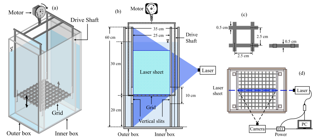
Figure 1 shows a schematic diagram of the experimental tank used in this study. This tank was made from transparent acrylic with an inner width $L$ of 25 cm and a height of 60 cm. The water depth measured from the center of the grid oscillation was fixed at 30 cm. Turbulence was generated in quiescent freshwater using a horizontal grid oscillated by a top-mounted motor, with a crank mechanism converted rotational motion into periodic vertical motion. The tank had a double-wall structure with two vertical inner walls separating the inner tank from the outer compartment. As shown in Figures 1(a) and (b),

Table 2: Experimental conditions

Run No.	f (Hz)	S (cm)	S/M (-)	Re (-)	SFP (-)
1	2.0	2.0	0.8	800	1
2	3.0			1200	1
3	4.0			1600	1
4	2.0	4.0	1.6	3200	2
5	3.0			4800	3
6	4.0			6400	3
7	2.0	6.0	2.4	7200	2
8	3.0			10800	2
9	4.0			14400	3

10-cm vertical slits were installed on the inner walls, through which the horizontal grid was connected to four driving shafts located in the outer compartment. Vertical oscillation of these shafts drove the grid motion. The center of the grid oscillation was located 20 cm above the tank bottom. The grid was fabricated using a 3D printer and consisted of square bars arranged in a square mesh shown in Figure 1(c), where the mesh size $M$ and the bar width $d$ were 2.5 cm and 0.5 cm, respectively.

In this study, three frequencies $f$ and three strokes $S$ were chosen, as summarized in Table 2. Here, $R e$ is the grid Reynolds number defined as $f S^{2} / ν$ , and SFP denotes the secondary-flow pattern classification, which will be defined in Section 3.1. The same grid was used throughout the present experiments; thus, the sizes of $M$ and $d$ remained constant.

2.2. PIV measurements

The PIV system shown in Figures 1(b) and (d) was used to measure the instantaneous velocity fields, which were calculated from successive particle images using image-correlation-based PIV analysis. Similar PIV-based measurements, including stereo-PIV, have been applied to resolve flow structures and momentum transport in previous studies^35,36). The freshwater in the tank was seeded with 100 μm reflective tracer particles with a specific gravity of 0.94. The PIV measurements were performed after sufficient mixing to ensure homogeneous particle seeding. A vertical laser sheet was used to illuminate the measurement plane by a 5 W continuous-wave semiconductor laser with a wavelength of 465 nm. Particle motions were continuously recorded by a high-speed camera with a resolution of 1,280 × 1,024 pixels. The frame rate was set to 200 Hz, providing an appropriate particle-image displacement for PIV cross-correlation. An interrogation window of 21 × 21 pixels, corresponding to approximately 0.5 cm × 0.5 cm, and a vector spacing of 0.25 cm were adopted, with about 50% overlap between adjacent windows.

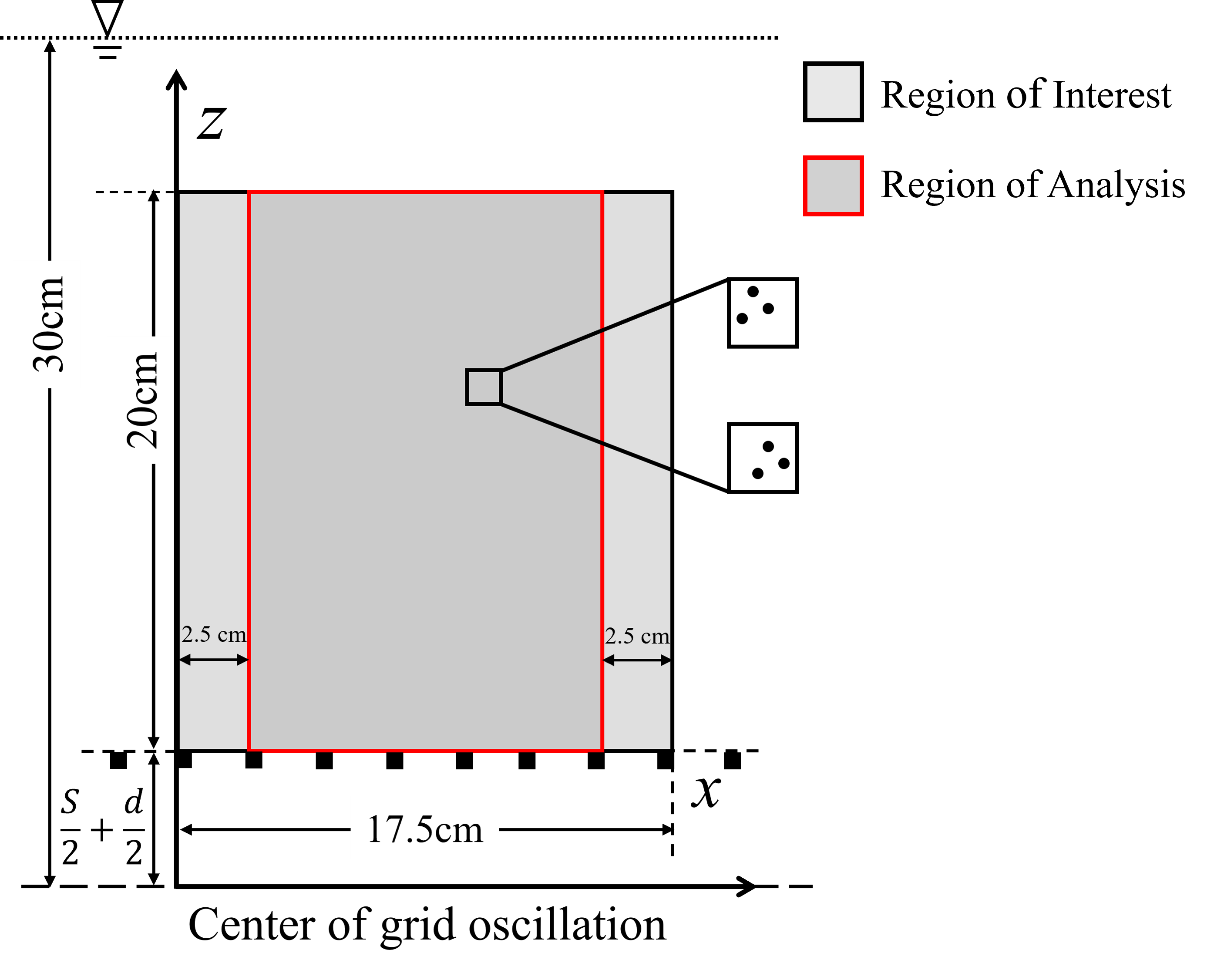
As shown in Figure 2, the region of interest (ROI) covered a 17.5 cm × 20 cm vertical section extending upward from the top surface of the grid at its upper stroke position. To minimize boundary effects and ensure a reliable characterization of the secondary flow, 2.5 cm-wide buffer regions on both sides were excluded from the statistical analysis. For each experimental condition, PIV measurements were started after an initial period of at least 3 min to allow the flow to develop. Subsequently, ten measurement runs, each lasting 20 s, were conducted while the grid continued to oscillate without interruption. During each measurement run, 4,000 consecutive images were captured. The cumulative data acquisition time over the ten runs was 200 s. The intervals between successive runs exceeded 2 min, and the ten runs spanned a total experimental duration exceeding 25 min.

Since the 2D-PIV measurements in this study cannot capture the out-of-plane velocity component and its spatial gradients, the complete three-dimensional turbulent kinetic energy and energy dissipation rate cannot be directly evaluated. The unmeasured terms in the energy dissipation rate were estimated by assuming horizontal isotropy together with the continuity equation. The resulting 2D-PIV-based estimates of the horizontal and vertical mean velocities $U$ and $W$ , horizontal and vertical turbulence intensities $u_{r m s}$ and $w_{r m s}$ , turbulent kinetic energy $k$ , and the energy dissipation rate $ε$ , are expressed as:

U = \frac{1}{N} \sum \bar{u}, W = \frac{1}{N} \sum \bar{w}

(3)

u_{r m s} = \frac{1}{N} \sum \sqrt{\bar{{u^{'}}^{2}}}, w_{r m s} = \frac{1}{N} \sum \sqrt{\bar{{w^{'}}^{2}}},

(4)

k = \frac{1}{N} \sum \frac{1}{2} {2 \bar{{u^{'}}^{2}} + \bar{{w^{'}}^{2}}},

(5)

ε = \frac{1}{N} \sum ν {\begin{matrix} 4.0 \bar{{(\frac{\partial u'}{\partial x})}^{2}} + 3.0 \bar{{(\frac{\partial u'}{\partial z})}^{2}} \\ + 3.0 \bar{{(\frac{\partial w'}{\partial x})}^{2}} + 4.0 \bar{{(\frac{\partial w'}{\partial z})}^{2}} \\ + 4.0 \bar{(\frac{\partial u'}{\partial x} \frac{\partial w'}{\partial z})} + 6.0 \bar{(\frac{\partial w'}{\partial x} \frac{\partial u'}{\partial z})} \end{matrix}} .

(6)

where $x$ and $z$ denote the horizontal and vertical coordinates, respectively. The quantities $u$ and $w$ represent the velocity components in their respective directions. The prime denotes fluctuating component from the time-averaged values, and the overbar indicates temporal averaging. In addition, $N$ is the number of individual ensemble runs. Eqs. (5) and (6), or their equivalent forms, have been widely used in previous 2D-PIV studies to estimate turbulent kinetic energy and the energy dissipation rate ^27,29,33).

In this study, in order to examine vertical profiles of turbulence statistics and the secondary velocity, we used the statistical quantities that were averaged spatially over the $x$ -direction, defined by ${⟨ \cdot ⟩}_{x}$ , as follows:

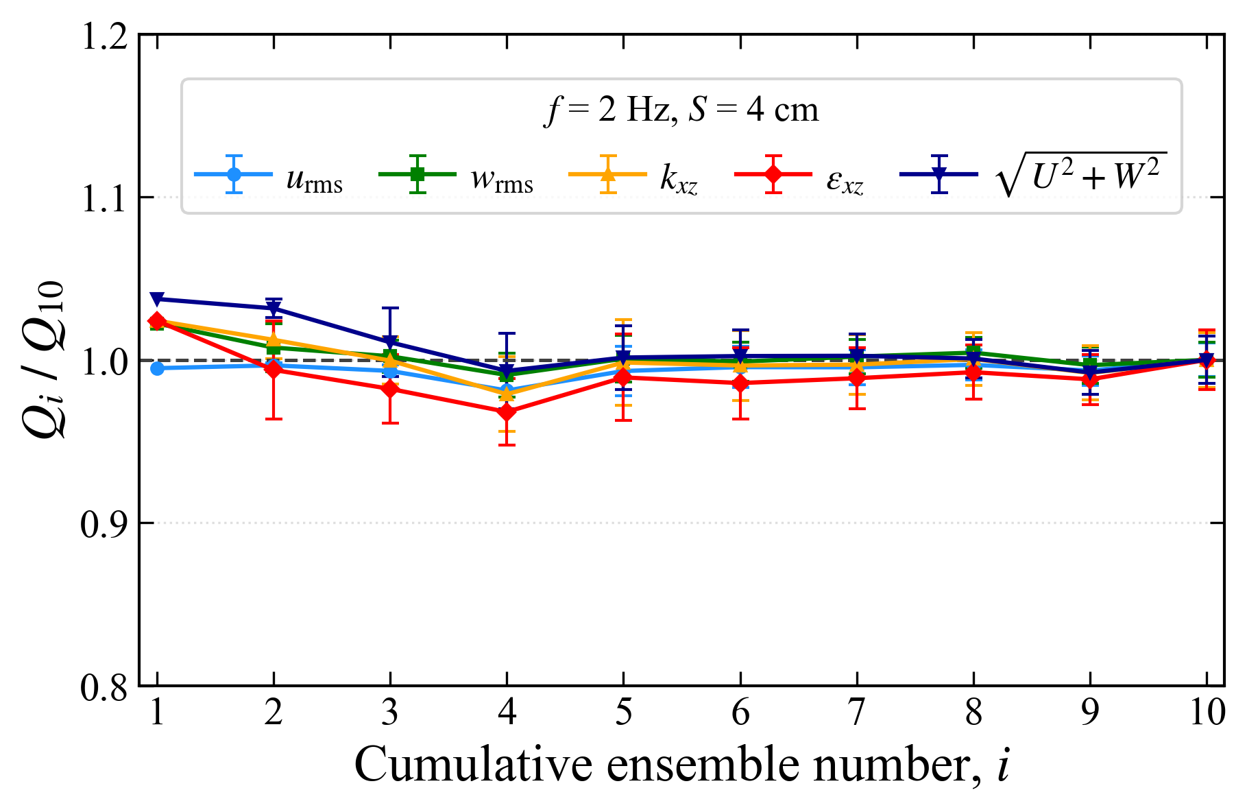
\begin{matrix} {U^{x} = ⟨ U ⟩}_{x}, & {W^{x} = ⟨ W ⟩}_{x}, \\ {u_{r m s}^{x} = ⟨ u_{r m s} ⟩}_{x}, & {w_{r m s}^{x} = ⟨ w_{r m s} ⟩}_{x}, \\ {k^{x} = ⟨ k ⟩}_{x}, & {ε^{x} = ⟨ ε ⟩}_{x} . \end{matrix}}

(7)

The statistical validity of the ten-run ensemble averaging was evaluated by progressively increasing the cumulative number of ensemble runs from 1 to 10. For the turbulence statistics, we introduced

Q_{i} = \frac{1}{i} \sum_{n = 1}^{i} {⟨ Q ⟩}_{x z}^{(n)}

(8)

Here, $Q_{i}$ denotes the cumulative ensemble average calculated from the first $i$ individual runs, where each run was first time-averaged and then spatially averaged over the $x$ - $z$ plane, expressed by ${⟨ \cdot ⟩}_{x z}$ . The ratio $Q_{i} / Q_{10}$ is used as an index of statistical convergence of the ensemble averaging from the first to the $i$ th run, where $Q_{10}$ represents the corresponding quantity obtained from all ten runs.

The case of $f = 2.0$ Hz and $S = 4.0$ cm was selected as a representative condition because it exhibited the largest horizontal inhomogeneity among all experimental conditions, as shown later in Figure 12. Figure 3 shows the variation of $Q_{i} / Q_{10}$ with the cumulative ensemble number for the turbulence statistics, i.e., $u_{r m s}$ , $w_{r m s}$ , $k$ , $ε$ , and the secondary-flow intensity $\sqrt{U^{2} + W^{2}}$ . All evaluated ratios approached approximately 1.0 as the cumulative ensemble number increased, indicating that the spatiotemporally averaged turbulence quantities and secondary-flow intensity were approximately converged within the ten-run ensemble. Therefore, the turbulence statistics obtained from the ten-run ensemble averaging were used in the subsequent analysis. However, this analysis provides only an approximate assessment of statistical convergence and does not capture the long-period variability of the secondary flows.

3. Results and Discussion

3.1. Classification of secondary-flow patterns

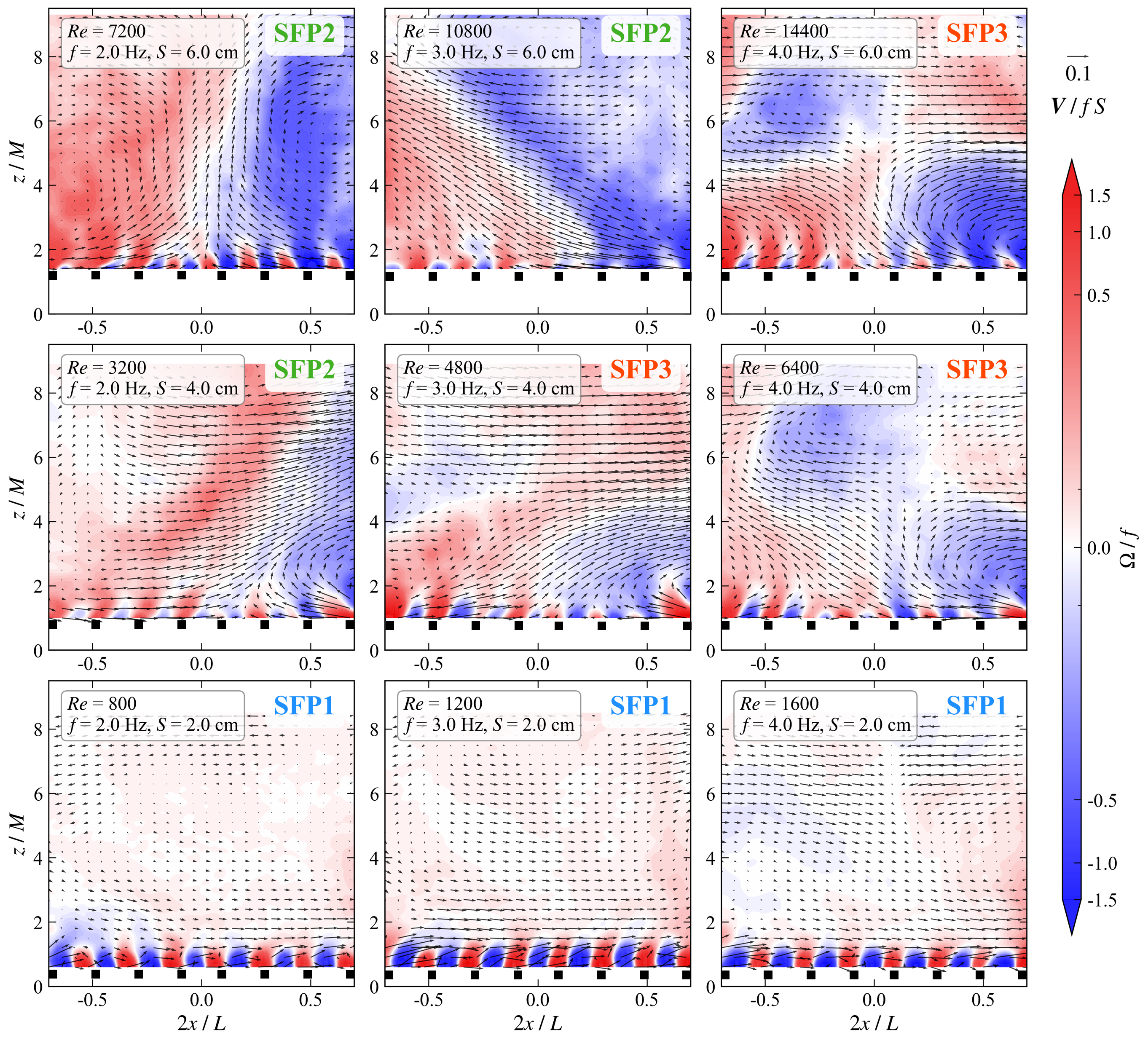
Figure 4 shows the spatial distributions of secondary-flow structures across a vertical cross-section at various Reynolds numbers together with the dimensionless horizontal vorticity of the secondary flows, $Ω / f$ . To make a systematic comparison under varying experimental conditions, the spatial coordinates are expressed as $2 x / L$ and $z / M$ , where $2 x / L = x / (L / 2$ ) represents the horizontal coordinate relative to the tank centerline, normalized by the half width of the inner tank because the spatial scale of the secondary flows is considered to depend on the tank scale. The secondary-flow velocity vector $𝑽$ is normalized by the grid-oscillation velocity scale $f S$ . In the Figures, the row of the black squares along the horizontal axis indicates the upper position of the grid. These Figures are systematically arranged so that the vertical direction represents the response of the flow structure to changes in $S$ , whereas the horizontal direction represents its response to changes in $f$ . Thus, the grid Reynolds number varies among the individual panels. It can be seen from Figure 4 that as the values of $f$ and $S$ vary, the secondary-flow fields visually exhibit three different spatial patterns, i.e., SFP1, SFP2 and SFP3.

First, SFP1 appears at $R e =$ 800, 1200 and 1600, where no clearly organized secondary-flow pattern is observed, though weak secondary motions still exist in the far-field region away from the grid. The SFP1 results indicate a rightward secondary flow near the grid, which is likely recirculated outside the analytical domain in either the vertical or spanwise direction. In contrast, the far-field region exhibits weak and complex secondary motions without a distinct closed circulation. In addition, the vorticity field around the grid exhibits alternating positive and negative regions, which are likely to represent organized small-scale vortices generated by the interaction of jets and wakes around the grid, as reported by Thompson and Turner²⁾. Significant vorticity and secondary-flow motions are almost confined to the region close to the grid, but weak secondary motions persist in the region away from the grid.

Next, SFP2 at $R e =$ 3200, 7200 and 10800 is discussed. In the SFP2 cases, a strong upward jet-like structure is observed near the center of the tank. The axis of this jet-like structure shifts from left to right depending on the grid-oscillation conditions, indicating that the large-scale flow structure may be unstable and sensitive to the forcing conditions. The case at $R e$ = 7200 is particularly representative, exhibiting a relatively symmetric upward-flow pattern. These results suggest that such a large-scale flow structure significantly influences the vertical distributions of turbulence statistics through turbulence production and the upward transport of turbulent energy from the oscillating grid.

Finally, a multiple-vortex secondary-flow pattern is observed in the SFP3 cases. The clearest example is found at $R e$ = 14400, where counterclockwise and clockwise circulations develop on the left and right sides of the tank's

lower layer, respectively, whereas an opposite circulation pattern may appear in the upper layer. This result suggests that the large-scale circulation extending over the entire water depth in SFP2 becomes structurally unstable with increasing Reynolds number and transitions into the multiple-vortex pattern.

As described above, the flow pattern changes with the grid Reynolds number, and the spatial structure of turbulence does not evolve monotonically. The development of large-scale secondary flows is therefore expected to significantly

**Fig. 3:** Convergence of turbulence statistics with increasing ensemble size

**Fig. 4:** Spatial distributions of secondary flows and horizontal vorticity

influence not only the spatial distribution of turbulence but also turbulence production and transport processes.

Asymmetric secondary-flow distributions were observed under some forcing conditions. Such asymmetry may result from several factors, including anisotropy induced by grid oscillation and near the tank corners, pressure fluctuations, and unavoidable slight asymmetries in the experimental apparatus. In addition, even a symmetric three-dimensional circulation may appear asymmetric in the present measurement plane if it is oriented obliquely with respect to the laser-light sheet. Similar nonsymmetric and unorganized horizontal mean flows were reported by McKenna and McGillis²⁹⁾ under forcing conditions with $S < 8$ cm. However, the present single-plane measurements cannot definitively identify the origin of the observed asymmetry. 3D-PIV or multi-plane measurements are required in future studies to examine the reproducibility and possible mechanisms underlying the asymmetry.

3.2. Relationship between turbulent kinetic energy and energy dissipation rate

With the exception of the studies by Matsunaga et al.²⁴⁾ and Poulain-Zarcos et al.²⁷⁾, measurements of the energy dissipation rate in oscillating-grid turbulence are still very scarce. Therefore, a comparison of the behaviors of turbulent kinetic energy and energy dissipation rate is of particular interest. Figure 5 shows the relationship between the turbulent kinetic energy $k^{x}$ and the dissipation rate $ε^{x}$ calculated from Eqs. (5) to (7). The turbulence measurements of Matsunaga et al.²⁴⁾ were performed using a traversing hot-film anemometer rather than PIV, and their data are also plotted in the Figure for comparison. It should be noted that only data from the region where turbulence remained relatively strong are presented; the power-law decay was expected to hold there ( $z / M \leq$ 2.5 for $S =$ 2.0 cm, and $z / M \leq$ 3.0 for $S =$ 4.0 cm and 6.0 cm), because the influence of secondary flows is considered to be relatively weak in this region compared to the grid forcing. Although both datasets exhibit a clear correlation between $ε^{x}$ and $k^{x}$ , the present data indicate a slightly gentler slope than that reported by Matsunaga et al.²⁴⁾. This may be attributed to the vertical decay behavior of the energy dissipation rate in this study, as will be explained in Section 3.3.

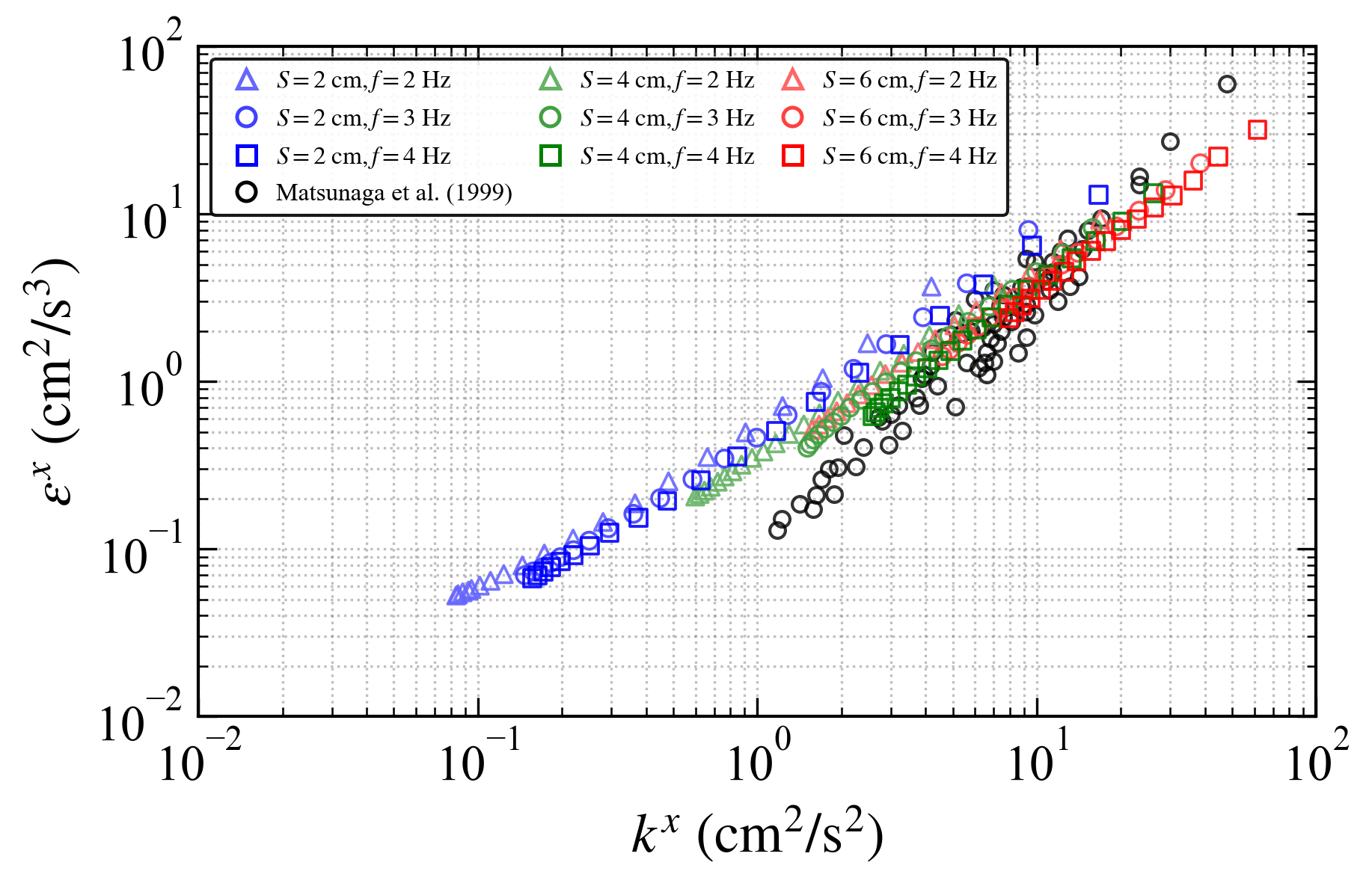
**Fig. 5:** Relationship between $k^{x}$ and $ε^{x}$

**Fig. 6:** Spatial distributions of (a) $k / f^{2} S^{2}$ and (b) $ε / f^{3} S^{2}$

Despite this difference, the magnitude of the present data is in reasonable agreement with their data in the relatively high-energy range, supporting the validity of the estimated energy dissipation rate in this study. However, the discrepancy between them implies that secondary-flow effects cannot be neglected even in regions where turbulence is relatively strong and may modify the vertical decay rates of turbulence statistics.

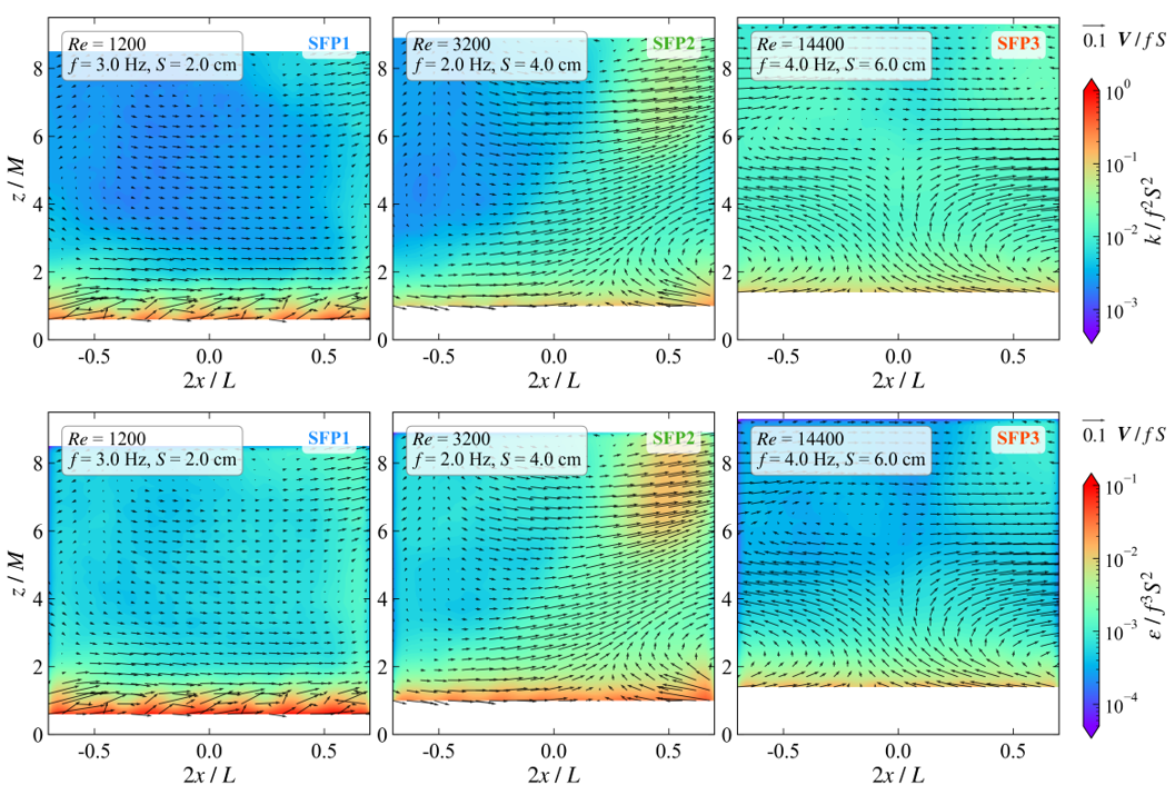
In Figure 6, the spatial distributions of the dimensionless turbulent kinetic energy $k^{x} / f^{2} S^{2}$ and the dimensionless energy dissipation rate $ε^{x} / f^{3} S^{2}$ are displayed for representative Reynolds numbers, corresponding to SFP1, SFP2, and SFP3. Both quantities exhibit qualitatively similar spatial patterns. The region close to the grid ( $z / M \leq$ 2.0) remains highly turbulent under all conditions. Far from the grid, their spatial distributions are influenced by the secondary flows. In SFP2, localized regions of high turbulent kinetic energy and energy dissipation rate are observed above the secondary-flow jet. These localized regions are likely formed by both turbulent transport and shear-induced turbulence production associated with the secondary flows. These results suggest that large-scale secondary flows redistribute turbulence and momentum generated by the grid oscillation, thereby significantly modifying the spatial distributions of the turbulent kinetic energy and the energy dissipation rate. Therefore, secondary flows are considered a primary factor reducing the isotropy and homogeneity of oscillating-grid turbulence.

3.3. Power-law scaling relations for turbulence statistics in strongly turbulent region

In order to extract the characteristics of oscillating-grid turbulence with minimal influence from secondary flows, the analysis provided in this section was restricted to regions relatively close to the grid, where turbulence remains strong. Following the approaches of Hopfinger and Toly⁹⁾, Ura et al.¹⁹⁾, and De Silva and Fernando²⁰⁾, the power-law scaling relations for turbulence statistics are assumed to be independent of the grid Reynolds number. However, as will be discussed later for the energy dissipation rate, some scatter attributable to Reynolds number effects was observed under relatively low-Reynolds-number conditions. In this study, turbulence statistics are assumed to depend on the oscillation frequency $f$ , the stroke $S$ , the mesh size $M$ , the bar width $d$ , and the distance from the center of the grid oscillation $z$ . Dimensional analysis therefore yields dimensionless turbulence statistics governed by the parameters $S / M$ , $d / M$ , and $z / M$ . Since $d / M$ was fixed at 0.2 in the present experiments, the dimensionless turbulence statistics, i.e., $u_{r m s}^{x} / f S$ , $w_{r m s}^{x} / f S$ , $k^{x} / f^{2} S^{2}$ and $ε^{x} / f^{3} S^{2}$ can be expressed as functions of $z / M$ and $S / M$ only.

**Fig. 7:** Power-law scaling relations of turbulence intensities in strongly turbulent region: (a) and (b) $z / M$ -dependence; (c) and (d) $S / M$ -dependence; (e) and (f) Normalized profiles

**Fig. 8:** Power-law scaling relations of turbulent kinetic energy and energy dissipation rate in strongly turbulent region:(a) and (b) $z / M$ -dependence; (c) and (d) $S / M$ -dependence; (e) and (f) Normalized profiles

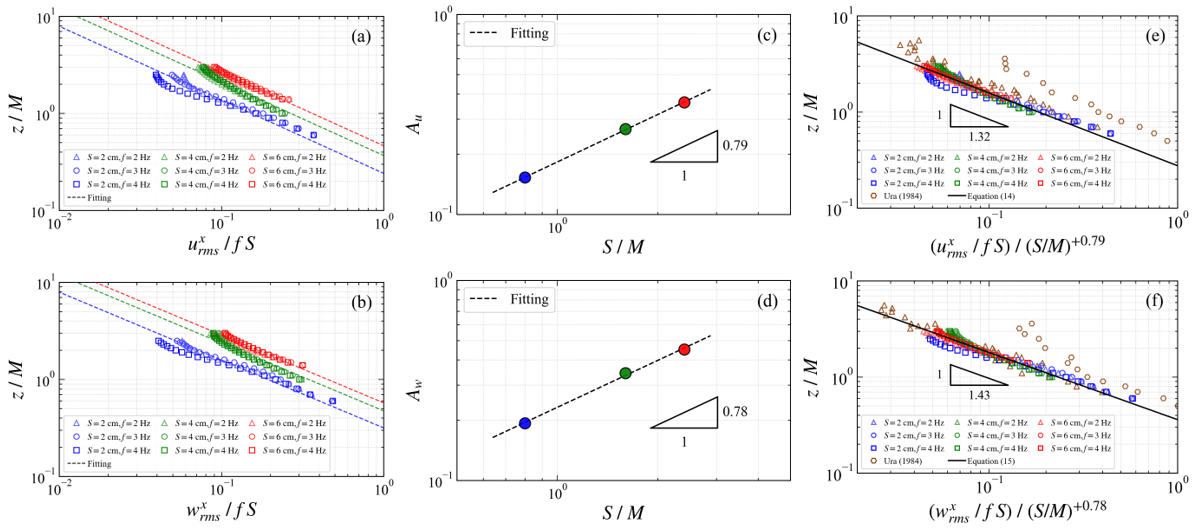
First, the power-law scaling relations for the vertical profiles of the turbulence intensities are quantified based on dimensional analysis. Figures 7(a) and (b) plot $u_{r m s}^{x} / f S$ and $w_{r m s}^{x} / f S$ against $z / M$ , with dashed-line fitting curves, respectively. These Figures show that both

quantities follow power-law scaling against $z / M$ within the range of $z / M \leq$ 2.5 for $S =$ 2.0 cm, and $z / M \leq$ 3.0 for $S =$ 4.0 cm and 6.0 cm. Based on these profiles, the empirical relations are expressed as

u_{r m s}^{x} / f S = A_{u} \times {(z / M)}^{- q_{u}},

(9)

w_{r m s}^{x} / f S = A_{w} \times {(z / M)}^{- q_{w}},

(10)

where the power-law exponents $q_{u}$ and $q_{w}$ were obtained from all the corresponding experimental data under the assumption that the respective exponents remain constant across all conditions as follows:

q_{u} = 1.32, q_{w} = 1.43 .

(11)

The coefficients $A_{u}$ and $A_{w}$ , which should depend on $S / M$ according to dimensional analysis, are plotted in Figures 7(c) and (d). These Figures show that the coefficients vary with the power of $S / M$ . The respective behaviors yield the following relations:

A_{u} \propto {(S / M)}^{0.79},

(12)

A_{w} \propto {(S / M)}^{0.78} .

(13)

Based on the results of Eqs. (9) to (13), the turbulence intensities are replotted against $z / M$ as shown in Figures 7(e) and (f) with the fitting curves. Here, the experimental data from Ura et al.¹⁹⁾ are also plotted for comparison. Therefore, in this study, the power-law relations in the strongly turbulent region for $u_{r m s}^{x} / f S$ and $w_{r m s}^{x} / f S$ are given by

u_{r m s}^{x} / f S = 0.183 {{(S / M)}^{0.79} (z / M)}^{- 1.32},

(14)

w_{r m s}^{x} / f S = 0.232 {{(S / M)}^{0.78} (z / M)}^{- 1.43} .

(15)

Although some of Ura's data show larger values than the present results, the overall decay trends are in good agreement with the present results. Also, the power-law exponents in Eqs. (14) and (15) are steeper than -1 reported by Hopfinger and Toly⁹⁾, and De Silva and Fernando²⁰⁾, but gentler than -1.5 reported by Thompson and Turner²⁾. Therefore, the proposed power-law relations for the turbulence intensities in the strongly turbulent region are consistent with those in previous studies.

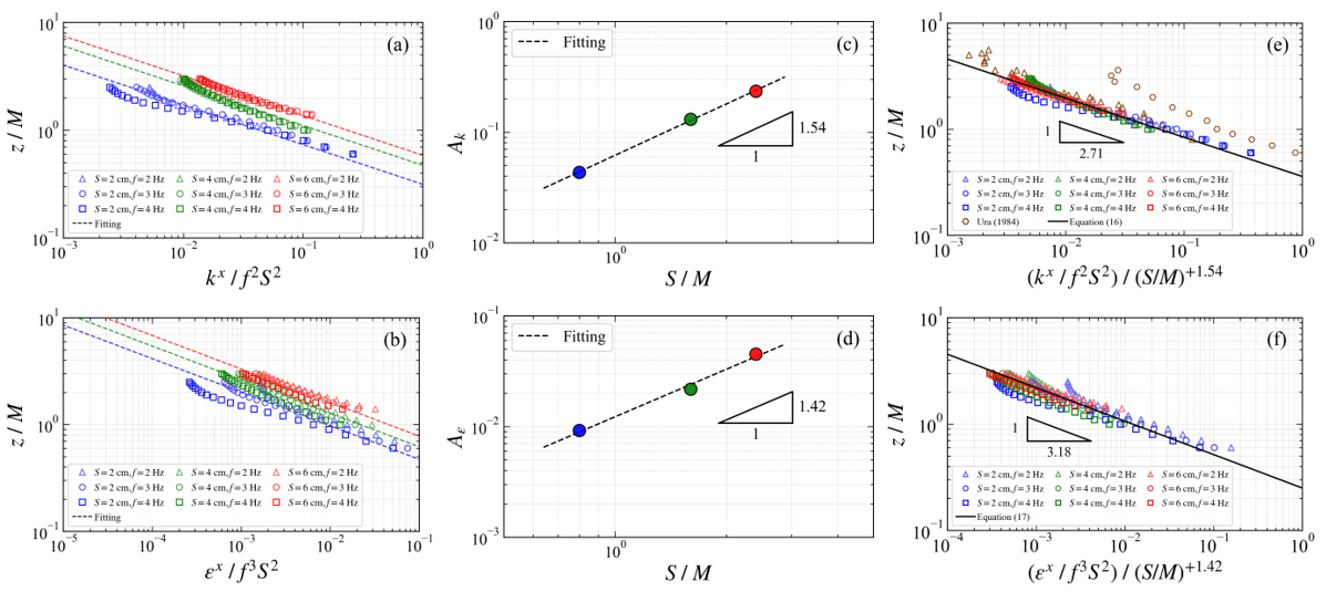
Following the procedure for the turbulence intensities, similar quantification was also applied to the dimensionless turbulent kinetic energy $k^{x} / f^{2} S^{2}$ and energy dissipation rate $ε^{x} / f^{3} S^{2}$ . The results are displayed in Figure 8, and the power-law scaling relations for $k^{x} / f^{2} S^{2}$ and $ε^{x} / f^{3} S^{2}$ as functions of $z / M$ and $S / M$ are finally expressed as

k^{x} / f^{2} S^{2} = 0.062 {{(S / M)}^{1.54} (z / M)}^{- 2.71},

(16)

ε^{x} / f^{3} S^{2} = 0.012 {{(S / M)}^{1.42} (z / M)}^{- 3.18} .

(17)

In the Figure of turbulent kinetic energy, the experimental data of Ura et al.¹⁹⁾ are also shown. Their data show considerable scatter; however, they appear to be in reasonable agreement with the present results. As can be seen from the definition of turbulent kinetic energy in Eq. (5), the power-law exponent for the turbulent kinetic energy is consistent with that estimated from Eqs. (14) and (15). On the other hand, the power-law exponent for the energy dissipation rate is gentler than the value of -4 reported in an earlier work³⁷⁾. This finding indicates that the influence of secondary flows may be more pronounced for the energy dissipation rate than for the other turbulence statistics, leading to deviations from the scaling behavior predicted by classical oscillating-grid turbulence theory. A physical reason for the smaller power-law exponent of the energy dissipation rate is not yet clear. However, secondary flows still exist even in the strongly turbulent region, and the energy dissipation rate, as a higher-order moment, may be more sensitive to small-scale structural changes in the turbulent field. This represents an interesting issue from the perspective of turbulence dynamics.

To assess the sensitivity associated with the horizontal isotropy assumption, analyses were conducted for both $k^{x}$ and $ε^{x}$ . The sensitivity of $k^{x}$ to the unmeasured y-direction turbulence component, i.e., $\bar{v'^{2}}$ , was evaluated by introducing a parameter $γ = \bar{v'^{2}} / \bar{u'^{2}}$ into Eq. (5). By varying $γ$ from 1.0 to 1.3, an approximately 10% change in $k^{x}$ was estimated under the present experimental conditions. In addition, the expression for the energy dissipation rate was compared between Eq. (6) and the following alternative expression:

ε_{1} = \frac{1}{N} \sum ν {\begin{matrix} 6.0 \bar{{(\frac{\partial u'}{\partial x})}^{2}} + 6.0 \bar{{(\frac{\partial u'}{\partial z})}^{2}} \\ + 6.0 \bar{(\frac{\partial w'}{\partial x} \frac{\partial u'}{\partial z})} \end{matrix}}

(18)

The corresponding value of $ε_{1}^{x} = ⟨ ε_{1} ⟩_{x}$ was then evaluated and compared with $ε^{x}$ . Using a similar parameterization to Eq. (17), the fitted power-law exponent associated with $S / M$ was 1.46, whereas the vertical power-law exponent associated with $z / M$ was −3.04, whose values are very similar to those in Eq. (17). These results indicate that the power-law scaling behavior and spatial characteristics of the estimated $k^{x}$ and $ε^{x}$ are not strongly sensitive to the degree of horizontal isotropy assumption. However, their magnitudes remain uncertain because they have not been validated against the corresponding three-dimensional quantities. We recognize that this limitation remains an important subject for future studies.

3.4. Vertical profiles of dimensionless turbulence statistics

The vertical profiles of the dimensionless mean velocities $U^{x} / f S$ and $W^{x} / f S$ are shown in Figure 9 to quantify the large-scale secondary flows. The dashed lines in the Figure indicate the overall vertical averages of these profiles. The error bars represent the standard deviations and are shown only for selected cases for visual clarity. In the SFP1 cases,

the profiles for both the horizontal and vertical dimensionless mean velocities become close to zero throughout the measurement region. This indicates that the grid-forcing energy is insufficient to generate a large-scale circulation, and the turbulence remains confined to the region near the grid. In the SFP2 and SFP3 cases, where

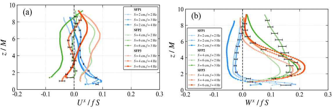
**Fig. 9:** Vertical profiles of dimensionless secondary flow velocities: (a) horizontal velocity and (b) vertical velocity

**Fig. 10:** Dimensionless vertical profiles of turbulence statistics based on the parametrizations: (a) $u_{r m s}^{x}$ , (b) $w_{r m s}^{x}$ , (c) $k^{x}$ and (d) $ε^{x}$

$f$ and $S$ are larger, the horizontal dimensionless velocity $U_{x} / f S$ is relatively weak, but the vertical one $W_{x} / f S$ increases substantially, exhibiting significant peaks around $z / M \approx$ 2 – 4. This transition indicates that the developing large-scale secondary flows in the measurement plane are primarily governed by vertical advection, with minimal influence on the horizontal mean flow.

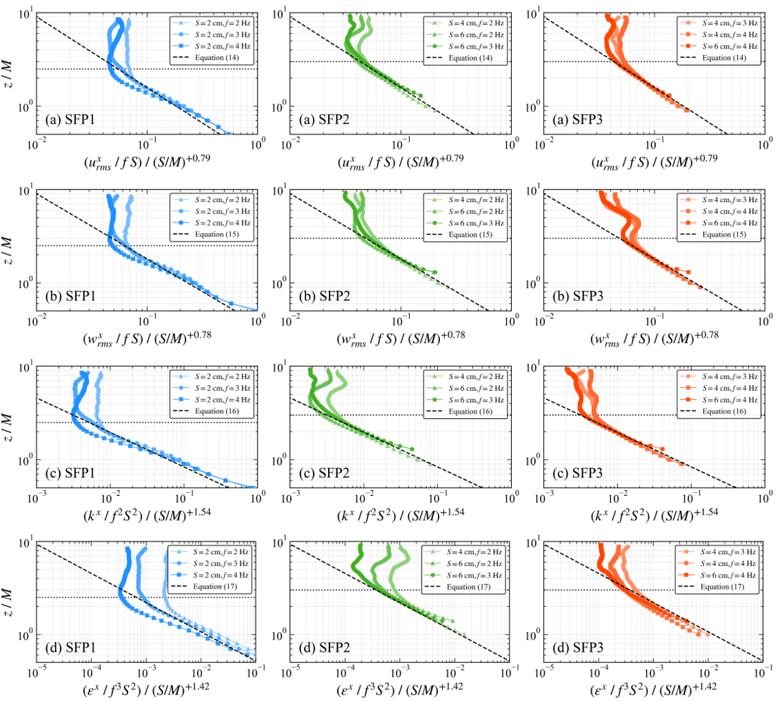
Figure 10 shows the vertical profiles of the dimensionless turbulence statistics, i.e., $u_{r m s}^{x}, w_{r m s}^{x}, k^{x}$ and $ε^{x}$ , grouped into SFP1-SFP3 according to the secondary-flow patterns. The dashed lines represent the respective power-law scaling relations by Eqs. (14) – (17). The dotted lines in the Figures also denote the application limits for the power-law relations. Regardless of the secondary-flow patterns, $u_{r m s}^{x}, w_{r m s}^{x},$ and $k^{x}$ in SFP1 follow their respective power-laws reasonably well in the region $z / M \leq$ 2.5. Moreover, under the stronger forcing conditions of the SFP2 and SFP3 cases, this valid range extends up to $z / M \leq$ 3.0. It is worth noting that, unlike the other turbulence statistics, $ε^{x}$ fails to collapse within the valid ranges of the power-law relations; in particular, the largest deviations are observed under low Reynolds number conditions in the SFP1 case. These results suggest that the energy dissipation rate is more susceptible to the Reynolds-number effects than the other turbulence statistics. A possible explanation is that the energy dissipation rate is calculated from spatial derivatives of fluctuating velocities (Eq. (6)) and therefore strongly reflects fine-scale turbulent structures. These fine-scale motions are considered to be relatively sensitive to Reynolds number effects. As a result, Reynolds-number dependence tends to appear more prominently only in the energy dissipation rate. Further investigations at more finely varied Reynolds numbers are required to clarify the underlying mechanisms.

Beyond the range where the power-law scaling applies, the turbulence statistics deviate from power-law behavior, no longer decay monotonically with distance from the grid, and instead show more complex profiles. The change in behavior suggests that, in the far-field region, turbulence production and transport associated with large-scale secondary flows become important processes, leading to deviations from the diffusion–dissipation balance of oscillating-grid turbulence. The change is most evident in the $w_{r m s}$ profile for the SFP3 cases, where local maxima appear in the far-field region. These maxima correspond closely to those of the vertical mean flow, suggesting that the vertical profiles of the turbulence statistics are significantly influenced by the spatial structure of the secondary flows.

Overall, the strongly turbulent region exhibits a largely universal power-law scaling governed primarily by the oscillating-grid forcing. Farther from the grid, however, the large-scale secondary flows increasingly redistribute the turbulent energy through turbulence production and vertical advection, resulting in gentler, but more complex vertical profiles. These results imply that the secondary-flow fields are less universal structures than those of oscillating-grid turbulence, leading to complex variability of the turbulence statistics in the far-field region.

**Fig. 11:** Isotropy ratio: (a) vertical distribution of ${〈 w_{r m s} / u_{r m s} 〉}_{x}$ , (b) horizontal distribution of ${〈 w_{r m s} / u_{r m s} 〉}_{z}$

**Fig. 12:** Horizontal homogeneity: (a) horizontal distribution of ${〈 u_{r m s} / u_{r m s}^{x} 〉}_{z}$ , (b) horizontal distribution of ${〈 w_{r m s} / w_{r m s}^{x} 〉}_{z}$

Quantifying the relative contributions of the grid forcing to the secondary flows remains an important subject in future study.

3.5. Isotropy ratio and horizontal homogeneity

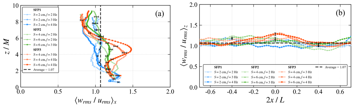
Figure 11 shows the vertical and horizontal distributions of the isotropy ratio ( $I R = w_{r m s} / u_{r m s}$ ), obtained by averaging in the horizontal and vertical directions, respectively. Here, ${⟨ \cdot ⟩}_{z}$ denotes the vertical mean value. Focusing on the vertical direction, ${〈 w_{r m s} / u_{r m s} 〉}_{x}$ remains close to 1.0 in SFP1, whereas pronounced peaks are observed around $z / M \approx$ 4.0–5.0 in SFP2 and SFP3, with the largest values occurring in SFP3. Farther from the grid, ${〈 w_{r m s} / u_{r m s} 〉}_{x}$ gradually returns to 1.0, and the vertically averaged value remains around 1.07, which is within the quasi-isotropic range reported in previous studies^7,9). In contrast, the horizontal distributions of ${〈 w_{r m s} / u_{r m s} 〉}_{z}$ are relatively uniform across all cases and remain close to the mean value 1.07. These results indicate that secondary flows primarily influence the vertical structure of turbulence in the measured $x - z$ plane, while the spatially averaged field remains largely horizontally homogeneous. It should be noted that $I R$ strictly quantifies the anisotropy between the vertical and horizontal velocity fluctuations rather than the anisotropy within the horizontal plane. Since the out-of-plane velocity component was not measured, the assumption of horizontal isotropy cannot be directly verified.

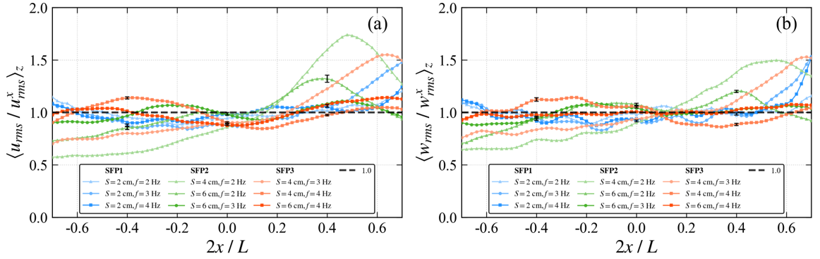
Figure 12 shows the horizontal homogeneity of the horizontal and vertical turbulence intensities, which are defined by ${〈 u_{r m s} / u_{r m s}^{x} 〉}_{z}$ and ${〈 w_{r m s} / w_{r m s}^{x} 〉}_{z}$ , respectively. They exhibit good horizontal uniformity within the central region of the tank. However, the turbulence intensity increases markedly near the right-side boundary ( $2 x / L > 0.2$ ), particularly in the SFP2 and SFP3 cases. The peak values reach approximately 1.7 and 1.5 for ${〈 u_{r m s} / u_{r m s}^{x} 〉}_{z}$ and ${〈 w_{r m s} / w_{r m s}^{x} 〉}_{z}$ , respectively, whereas substantially lower values are observed on the opposite side.

The persistence of asymmetric distributions in the ten-run ensemble averages suggests that they are not simply caused by random fluctuations of large-scale secondary-flow structures. As discussed in Section 3.1, this asymmetry may originate from a three-dimensional secondary-flow structure oriented obliquely with respect to the laser-light sheet, or alternatively, may be attributed to the amplification of unavoidable asymmetries in the experimental apparatus under grid oscillation. Previous studies of oscillating-grid experiments have similarly reported asymmetric mean flows even under small-stroke forcing^29,34). However, the present single-plane measurements cannot identify the precise cause. Future 3D-PIV or multi-plane measurements are required to determine the origin and reproducibility of this asymmetry in the turbulence statistics and secondary-flow structures.

4. Conclusions

This study experimentally investigated the effects of secondary flows on oscillating-grid turbulence. PIV measurements were conducted over a wide range of experimental conditions, and nine experimental cases were classified into three secondary-flow patterns. These patterns evolved from turbulence localized near the grid (SFP1), through a regime characterized by a structurally unstable and condition-sensitive, depth-scale upward jet (SFP2), to a state dominated by multiple secondary circulations (SFP3).

In the near-grid region of relatively strong turbulence, power-law scaling was observed for the turbulence statistics. The power-law scaling relations for the turbulence statistics, i.e., the horizontal and vertical turbulence intensities, turbulent kinetic energy, and energy dissipation rate, were quantitatively evaluated as functions of the dimensionless vertical coordinate $z / M$ and the grid parameter $S / M$ , and were compared with the results of previous studies. However, in the SFP1 cases, the energy dissipation rate did not exhibit universal scaling even in the strongly turbulent region, indicating a Reynolds-number dependence. In addition, the weaker vertical decay of the dissipation rate suggested that it was more sensitive to the secondary-flow structures than the other turbulence statistics. In contrast, in the far-field region away from the grid, all the turbulence statistics deviated from the power-law scaling and instead showed more complex profiles depending on the secondary-flow structures. This change in behavior suggests that, away from the grid, the turbulence production and transport associated with large-scale secondary flows became increasingly important from SFP1 to SFP3, leading to deviations from the diffusion–dissipation balance characteristic of oscillating-grid turbulence.

Although the sensitivity analysis suggested that the power-law scaling relations and spatial distributions of $k^{x}$ and $ε^{x}$ were not strongly dependent on the degree of horizontal isotropy assumption, their magnitudes remain uncertain. Furthermore, the isotropy ratio and horizontal homogeneity of the turbulent field were analyzed. The results of the present study showed that the isotropy ratio strongly depends on the spatial structures of large-scale secondary flows. In addition, the development of large-scale secondary flows progressively disrupted the horizontal homogeneity of oscillating-grid turbulence.

Overall, the present results demonstrate that the secondary-flow patterns represented by SFP1–SFP3 are important factors governing the vertical profiles and scaling behavior of the turbulence statistics in a confined oscillating-grid tank. These findings underscore the importance of explicitly accounting for secondary-flow effects in understanding the structure of oscillating-grid turbulence and in developing its parameterizations. Future work should focus on clarifying the three-dimensional structures and origins of the secondary flows using 3D-PIV or multi-plane measurements, as well as investigating their characteristic timescales and long-period variability through longer continuous measurements.

Acknowledgements

This work was partially supported by a Grant-in-Aid for Scientific Research (B) (JSPS KAKENHI Grant Number JP23K26211) and the collaborative research program (2026GC-05) of the Disaster Prevention Research Institute of Kyoto University.

Nomenclature

Symbol	Description (Unit)
A_u, A_w, A_k, A_ε	experimental constant (–)
C_u, C_w	experimental constant (–)
d	grid bar width (cm)
f	grid frequency (Hz)
i	cumulative number of ensemble runs (–)
$k$	2D-PIV-based estimate of turbulent kinetic energy (cm²s^-2)
L	tank inner width (cm)
M	grid mesh size (cm)
N	total number of ensemble runs (–)
q_u, q_w	power-law decay exponent (–)
Q_i/Q₁₀	statistical convergence ratio (–)
Re	grid Reynolds number (–)
S	grid stroke (cm)
u_rms,w_rms	turbulence intensity (cm s^-1)
u', v', w'	fluctuating velocity (cm s^-1)
U,W	mean velocity (cm s^-1)
V	secondary-flow velocity vector (cm s^-1)
x, y, z	horizontal and vertical coordinates (cm)

Greek symbols

Symbol	Description (Unit)
$γ$	ratio of horizontal velocity variances (–)
$ε, ε_{1}$	2D-PIV-based estimate of energy dissipation rate (cm²s^-3)
$ν$	kinematic viscosity (cm²s^-1)
Ω	horizontal vorticity for secondary flow (s^-1)

Subscripts

Symbol	Description (Unit)
${⟨ \cdot ⟩}_{x}$	x-direction averaged
${⟨ \cdot ⟩}_{x z}$	x-z plane averaged
${⟨ \cdot ⟩}_{z}$	z-direction averaged

References

H. Rouse and J. Dodu, "Turbulent diffusion across a density discontinuity," La Houille Blanche., 4 522-532 (1955). doi:10.1051/lhb/1955050.
S. M. Thompson and J. S. Turner, "Mixing across an interface due to turbulence generated by an oscillating grid," J. Fluid Mech., 67 (2) 349-368 (1975). doi:10.1017/S0022112075000341.
G. T. Csanady, "Air-Sea Interaction: Laws and Mechanisms," Cambridge University Press, (2001) https://books.google.co.in/books?id=slDSDyw-Gv8C.
P. P. Sullivan and J. C. McWilliams, "Dynamics of winds and currents coupled to surface waves," Annu. Rev. Fluid Mech., 42 19-42 (2010). doi:10.1146/annurev-fluid-121108-145541.
I. Nezu and K. Onitsuka, “Turbulent structures in partly vegetated open-channel flows with LDA and PIV measurements,” J. Hydraul. Res., 39 (6) 629–642 (2001). doi:10.1080/00221686.2001.9628292.
J. Yan, N. S. Cheng, H. W. Tang and S. K. Tan, "Oscillating-grid turbulence and its applications: a review," J. Hydraul. Res., 45 (1) 26-32 (2007). doi:10.1080/00221686.2007.9521740.
I. P. D. De Silva and H. J. S. Fernando, "Oscillating grids as a source of nearly isotropic turbulence," Phys. Fluids., 6 (7) 2455-2464 (1994). doi:10.1063/1.868193.
A. Eidelman, T. Elperin, A. Kapusta, N. Kleeorin, A. Krein and I. Rogachevskii, "Oscillating grids turbulence generator for turbulent transport studies," Nonlin. Processes Geophys., 9 201-205 (2002). doi:10.5194/npg-9-201-2002.
E. J. Hopfinger and J.-A. Toly, "Spatially decaying turbulence and its relation to mixing across density interfaces," J. Fluid Mech., 78 (1) 155-175 (1976). doi:10.1017/S0022112076002371.
J. S. Turner, "The influence of molecular diffusivity on turbulent entrainment across a density interface," J. Fluid Mech., 33 (4) 639-656 (1968). doi:10.1017/S002211206800159X.
P. F. Linden, "Mixing across a density interface produced by grid turbulence," J. Fluid Mech., 100(4), 691-703 (1980). doi:10.1017/S002211208000136X.
Y. Nakamura, M. Murai, T. Komatsu, E. Aburajima, T. Inoue and T. Shibata, “Experimental research on gas exchange mechanism using minute oxygen electrode,” Annu. J. Coast. Eng., JSCE, 44 (2) 1236–1240 (1997) doi:10.2208/proce1989.44.1236 (in Japanese).
H. Tsumori and Y. Sugihara, "Lengthscales of motions that control air–water gas transfer in grid-stirred turbulence," J. Mar. Syst., 66 (1-4) 6-18 (2007). doi:10.1016/j.jmarsys.2006.03.018.
Herlina and G. H. Jirka, "Experiments on gas transfer at the air-water interface induced by oscillating grid turbulence," J. Fluid Mech., 594 183-208 (2008). doi:10.1017/S0022112007008968.
H. E. Schulz and J. G. Janzen, "Concentration fields near air-water interfaces during interfacial mass transport: oxygen transport and random square wave analysis," Braz. J. Chem. Eng., 26 (3), 527-536 (2009). doi:10.1590/S0104-66322009000300008.
M. Rastello, H. Michallet, and J. L. Marié, "Sediment erosion in zero-mean-shear turbulence," Phys. Fluids., 32 (3) 036601 (2020). doi:10.1063/1.5141943.
M. Tamai, K. Muraoka, and K. Shimizu, "Study on interaction between turbulence generated by uniformly falling particles and oscillating grid turbulence," Proc. JSCE., No. 521/Ⅱ-32, 49-58 (1995) (in Japanese).
D. Pujol, J. Colomer, T. Serra, and X. Casamitjana, "A model for the effect of submerged aquatic vegetation on turbulence induced by an oscillating grid," Estuar. Coast. Shelf Sci., 114 23-30 (2012). doi:10.1016/j.ecss.2011.08.020.
M. Ura, T. Komatsu and N. Matsunaga, "Interfacial properties and entrainment due to turbulence generated by an oscillating grid," Proc. JSCE., 345(II-1) 91-99 (1984) (in Japanese).
I. P. D. De Silva and H. J. S. Fernando, "Some aspects of mixing in a stratified turbulent patch," J. Fluid Mech., 240 601-625 (1992). doi:10.1017/S0022112092000223.
R. I. Nokes, "On the entrainment rate across a density interface," J. Fluid Mech., 188 185-204 (1988). doi:10.1017/S0022112088000692.
N.-S. Cheng and A. W.-K. Law, "Measurements of turbulence generated by oscillating grid," J. Hydraul. Eng., 127 (3) 201-208 (2001). doi:10.1061/(ASCE)0733-9429(2001)127:3(201).
T. J. McDougall, "Measurements of turbulence in a zero-mean-shear mixed layer," J. Fluid Mech., 94(3) 409-431 (1979). doi:10.1017/S0022112079001105.
N. Matsunaga, Y. Sugihara, T. Komatsu and A. Masuda, "Quantitative properties of oscillating-grid turbulence in a homogeneous fluid," Fluid Dyn. Res., 25 (3) 147-165 (1999). doi:10.1016/S0169-5983(98)00034-3.
W. K. George, H. Wang, C. Wollblad and T. G. Johansson, "Homogeneous turbulence and its relation to realizable flows," Proc. 14th Australasian Fluid Mechanics Conf., Adelaide, Australia, 41-48 (2001).
W.H.M. Wan Mohtar, "Oscillating-grid turbulence at large strokes: Revisiting the equation of Hopfinger and Toly," J. Hydrodyn., 28 (3) 473-481 (2016). doi:10.1016/S1001-6058(16)60651-0.
M. Poulain-Zarcos, M. J. Mercier and A. ter Halle, "Global characterization of oscillating grid turbulence in homogeneous and two-layer fluids, and its implication for mixing at high Peclet number," Phys. Rev. Fluids., 7 054606 (2022). doi:10.1103/PhysRevFluids.7.054606.
H. J. S. Fernando and I. P. D. De Silva, "Note on secondary flows in oscillating-grid, mixing-box experiments," Phys. Fluids., 5 (7) 1849-1851 (1993). doi:10.1063/1.858808.
S. P. McKenna and W. R. McGillis, "Observations of flow repeatability and secondary circulation in an oscillating grid-stirred tank," Phys. Fluids., 16 (9) 3499-3502 (2004). doi:10.1063/1.1779671.
A. Srdic, H. J. S. Fernando and L. Montenegro, "Generation of nearly isotropic turbulence using two oscillating grids," Exp. Fluids, 20 395-397 (1996). doi:10.1007/BF00191022.
H. Matinpour, J. Atkinson and S. Bennett, "Secondary circulation within a mixing box and its effect on turbulence," Exp. Fluids., 61 225 (2020). doi:10.1007/s00348-020-03064-9.
V. Musy, A. Hantson, D. Thomas, J. C. Baudez and T. Lacassagne, "Experimental characterization of the flow and turbulence generated by fractal oscillating grids," Phys. Fluids, 36 (10) 105162 (2024). doi:10.1063/5.0228992.
M. W. McCorquodale and R. J. Munro, "Experimental study of oscillating-grid turbulence interacting with a solid boundary," J. Fluid Mech., 813 768-798 (2017). doi:10.1017/jfm.2016.843.
M. W. McCorquodale and R. J. Munro, "A method for reducing mean flow in oscillating-grid turbulence," Exp. Fluids., 59 182 (2018). doi:10.1007/s00348-018-2636-7.
K. Takehara, R. J. Adrian, G. T. Etoh and K. T. Christensen, “A Kalman tracker for super-resolution PIV,” Exp. Fluids., 29 (Suppl. 1) S034-S041 (2000). doi:10.1007/s003480070005.
H. Aita, R. Hirakawa and T. Ohmoto, “Stereo-PIV measurements of flow at boundary of spur dikes,” Jpn. J. JSCE., 82 (15) 25-15048 (2026). doi:10.2208/jscejj.25-15048 (in Japanese).
D.H. Bache and E. Rasool, "Measurement of the rate of energy dissipation around an oscillating grid by an energy balance approach," Chem. Eng. J. Biochem. Eng. J., 63 (2) 105-115 (1996). doi:10.1016/0923-0467(96)03077-1.